Möbius transformation
- Möbius transformations should not be confused with the Möbius transform or the Möbius function.
In geometry, a Möbius transformation is a rational function of the form:
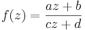
where z, a, b, c, d are complex numbers satisfying ad − bc ≠ 0. Möbius transformations are named in honor of August Ferdinand Möbius, although they are also called homographic transformations, linear fractional transformations, or fractional linear transformations.
Overview
A Möbius transformation is a bijective conformal map of the extended complex plane (i.e. the complex plane augmented by the point at infinity, also known as Riemann sphere):
The set of all Möbius transformations forms a group under composition called the Möbius group.
The Möbius group is the automorphism group of the Riemann sphere, sometimes denoted

Certain subgroups of the Möbius group form the automorphism groups of the other simply-connected Riemann surfaces (the complex plane and the hyperbolic plane). As such, Möbius transformations play an important role in the theory of Riemann surfaces. The fundamental group of every Riemann surface is a discrete subgroup of the Möbius group (see Fuchsian group and Kleinian group). Möbius transformations are also closely related to isometries of hyperbolic 3-manifolds.
A particularly important subgroup of the Möbius group is the modular group; it is central to the theory of many fractals, modular forms, elliptic curves and Pellian equations.
In physics, the identity component of the Lorentz group acts on the celestial sphere the same way that the Möbius group acts on the Riemann sphere. In fact, these two groups are isomorphic. An observer who accelerates to relativistic velocities will see the pattern of constellations as seen near the Earth continuously transform according to infinitesimal Möbius transformations. This observation is often taken as the starting point of twistor theory.
Definition
The general form of a Möbius transformation is given by
where a, b, c, d are any complex numbers satisfying ad − bc ≠ 0. (If ad = bc the rational function defined above is a constant.) This definition can be extended to the whole Riemann sphere (the complex plane plus the point at infinity).
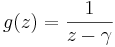
The set of all Möbius transformations forms a group under composition. This group can be given the structure of a complex manifold in such a way that composition and inversion are holomorphic maps. The Möbius group is then a complex Lie group. The Möbius group is usually denoted  as it is the automorphism group of the Riemann sphere.
Decomposition and elementary properties
A Möbius transformation is equivalent to a sequence of simpler transformations. Let:
 (translation)
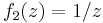 (inversion and reflection)
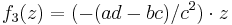 (dilation and rotation)
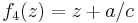 (translation)
then these functions can be composed on each other, giving
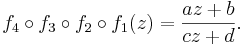
This decomposition makes many properties of the Möbius transform obvious.
For example, the preservation of angles is reduced to proving the angle preservation property of circle inversion, since all other transformation are dilations or isometries, which trivially preserve angles.
The existence of an inverse Möbius transformation function and its explicit formula is easily derived by a composition of the inverse function of the simpler transformations. That is, define functions  such that
  is the inverse of
  , then composition
  would be the explicit expression for the inverse Möbius transformation:

From this decomposition, we also see that Möbius transformation carries over all non-trivial properties of circle inversion. Namely, that circles are mapped to circles, and angles are preserved. Also, because of the circle inversion, is carried over the convenience of defining Möbius transformation over a plane with a point at infinity, which makes statements and concepts of Möbius transformation's properties simpler.
For another example, look at  . If
. If  , then the transformation collapses to the point 0, then
  moves to
  . Collapsing to a point is not an interesting transformation, thus we require in the definition of Möbius transformation that
  .
.
Preservation of angles and circles
As seen from the above decomposition, Möbius transformation contains this transformation  , called complex inversion. Geometrically, a complex inversion is a circle inversion followed by a reflection around the x-axis.
In circle inversion, circles are mapped to circles (here, lines are considered as circles with infinite radius), and angles are preserved. See circle inversion for various properties and proofs.
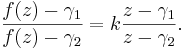
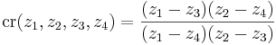
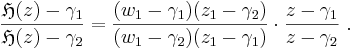
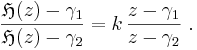
Cross-ratio preservation
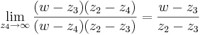
The cross-ratio preservation theorem states that the cross-ratio
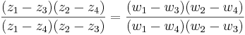
is invariant under a Möbius transformation that maps from z to w.
The action of the Möbius group on the Riemann sphere is sharply 3-transitive in the sense that there is a unique Möbius transformation which takes any three distinct points on the Riemann sphere to any other set of three distinct points. See the section below on specifying a transformation by three points.
Projective matrix representations
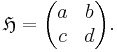
The transformation
is determined by the matrix of complex numbers
The condition ad − bc ≠ 0 is equivalent to the condition that the determinant of above matrix be nonzero (i.e. the matrix should be non-singular). Note that any matrix obtained by multiplying  by a complex scalar λ determines the same transformation, so the transformation does not determine the matrix. The freedom of choosing the matrix for a given transformation can be restricted by requiring that the determinant of be equal to 1; then will be unique up to sign.
The usefulness of using matrices to describe Möbius transformations stems from the fact that matrix multiplication gives rise to composition of the corresponding Möbius transformations. In other words, the map
from the general linear group GL(2,C) to the Möbius group, which sends the matrix  to the transformation f is a group homomorphism. This map is called a projective representation of GL(2,C) for reasons explained below.
The map  is not an isomorphism, since it maps any scalar multiple of to the same transformation. The kernel of this homomorphism is then the set of all scalar multiples of the identity matrix, which is the center Z(GL(2,C)) of GL(2,C). The quotient group GL(2,C)/Z(GL(2,C)) is called the projective linear group and is usually denoted PGL(2,C). By the first isomorphism theorem of group theory we conclude that the Möbius group is isomorphic to PGL(2,C). Since Z(GL(2,C)) is the kernel of the group action given by GL(2,C) acting on itself by conjugation, PGL(2, C) is isomorphic to the inner automorphism group of GL(2,C). Moreover, the natural action of PGL(2,C) on the complex projective line CP1 is exactly the natural action of the Möbius group on the Riemann sphere, where the projective line CP1 and the Riemann sphere are identified as follows:
![[z_1�: z_2]\leftrightarrow z_1/z_2.](/2009-wikipedia_en_wp1-0.7_2009-05/I/0d5cef6faf5445861e5c9d7264c11a7c.png)
Here [z1:z2] are homogeneous coordinates on CP1; the point [1:0] corresponds to the point ∞ of the Riemann sphere.
If one restricts to matrices of determinant one, the map restricts to a surjective map from the special linear group SL(2,C) to the Möbius group; in the restricted setting the kernel (formed by plus and minus the identity) is still the center of the group. The Möbius group is therefore also isomorphic to PSL(2,C). We then have the following isomorphisms:

From the last identification we see that the Möbius group is a 3-dimensional complex Lie group (or a 6-dimensional real Lie group).
Note that there are precisely two matrices with unit determinant which can be used to represent any given Möbius transformation. That is, SL(2,C) is a double cover of PSL(2,C). Since SL(2,C) is simply-connected it is the universal cover of the Möbius group. Therefore the fundamental group of the Möbius group is Z2.
Classification
Möbius transformations are commonly classified into four types, parabolic, elliptic, hyperbolic and loxodromic (actually hyperbolic is a special case of loxodromic). The classification has both algebraic and geometric significance. Geometrically, the different types result in different transformations of the complex plane, as the figures below illustrate. These types can be distinguished by looking at the trace  . Note that the trace is invariant under conjugation, that is,
and so every member of a conjugacy class will have the same trace. Every Möbius transformation can be written such that its representing matrix has determinant one (by multiplying the entries with a suitable scalar). Two Möbius transformations  (both not equal to the identity transform) with
  are conjugate if and only if
  .
.
In the following discussion we will always assume that the representing matrix is normalized such that  .
.
Parabolic transforms
A non-identity Möbius transformation defined by a matrix of determinant one is said to be parabolic if
(so the trace is plus or minus 2; either can occur for a given transformation since is determined only up to sign). In fact one of the choices for has the same characteristic polynomial X2−2X+1 as the identity matrix, and is therefore unipotent. A Möbius transform is parabolic if and only if it has exactly one fixed point in the compactified complex plane 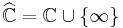 , which happens if and only if it can be defined by a matrix conjugate to

The set of all parabolic Möbius transformations with a given fixed point in  , together with the identity, forms a subgroup isomorphic to the group of matrices

for  ; this is an example of a Borel subgroup (of the Möbius group, or of SL(2,C) for the matrix group; the notion is defined for any reductive Lie group).
All other non-identity transformations have two fixed points. All non-parabolic (non-identity) transformations are defined by a matrix conjugate to
with  not equal to 0, 1 or −1. The square
  is called the characteristic constant or multiplier of the transformation.
Elliptic transforms
The transformation is said to be elliptic if it can be represented by a matrix whose trace is real with
A transform is elliptic if and only if  . Writing
  , an elliptic transform is conjugate to
with  real. Note that for any with characteristic constant k, the characteristic constant of
  is
is  . Thus, the only Möbius transformations of finite order are the elliptic transformations, and these only when λ is a root of unity; equivalently, when α is a rational multiple of π.
Hyperbolic transforms
The transform is said to be hyperbolic if it can be represented by a matrix whose trace is real with

A transform is hyperbolic if and only if λ is real and positive.
Loxodromic transforms
The transform is said to be loxodromic if  is not in [0,∞). A transformation is loxodromic if and only if
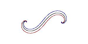
  . Historically, navigation by loxodrome or rhumb line refers to a path of constant bearing; the resulting path is a logarithmic spiral, similar in shape to the transformations of the complex plane that a loxodromic Möbius transformation makes. See the geometric figures below.
| Transformation | Trace squared | Multipliers | Class representative | |
|---|---|---|---|---|
| Elliptic |  |
  |
 |
 |
| Parabolic |  |
 |
 |
 |
| Hyperbolic |  |
  |
 |
 |
| Loxodromic |  |
  |
 |
 |
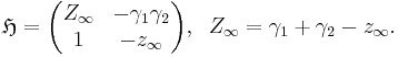
Fixed points
Every non-identity Möbius transformation has two fixed points  on the Riemann sphere. Note that the fixed points are counted here with multiplicity; for parabolic transformations, the fixed points coincide. Either or both of these fixed points may be the point at infinity.
The fixed points of the transformation
are obtained by solving the fixed point equation  . For
. For  , this has two roots (proof):

Note that for parabolic transformations, which satisfy  , the fixed points coincide.
When c = 0, one of the fixed points is at infinity; the other is given by
The transformation will be a simple transformation composed of translations, rotations, and dilations:
If c = 0 and a = d, then both fixed points are at infinity, and the Möbius transformation corresponds to a pure translation:  .
.
Normal form
Möbius transformations are also sometimes written in terms of their fixed points in so-called normal form. We first treat the non-parabolic case, for which there are two distinct fixed points.
Non-parabolic case:
Every non-parabolic transformation is conjugate to a dilation, i.e. a transformation of the form
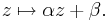
with fixed points at 0 and ∞. To see this define a map
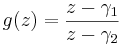
which sends the points  to
to  . Here we assume that both
  and
and  are finite. If one of them is already at infinity then g can be modified so as to fix infinity and send the other point to 0.
If f has distinct fixed points then the transformation  has fixed points at 0 and ∞ and is therefore a dilation:
 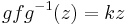 . The fixed point equation for the transformation f can then be written
Solving for f gives (in matrix form):

or, if one of the fixed points is at infinity:
From the above expressions one can calculate the derivatives of f at the fixed points:
 and
and 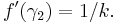
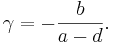
Observe that, given an ordering of the fixed points, we can distinguish one of the multipliers (k) of f as the characteristic constant of f. Reversing the order of the fixed points is equivalent to taking the inverse multiplier for the characteristic constant:

For loxodromic transformations, whenever  , one says that is the repulsive fixed point, and is the attractive fixed point. For
  , the roles are reversed.
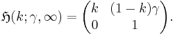
Parabolic case:
In the parabolic case there is only one fixed point  . The transformation sending that point to ∞ is
or the identity if is already at infinity. The transformation fixes infinity and is therefore a translation:
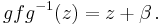
Here, β is called the translation length. The fixed point formula for a parabolic transformation is then
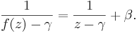
Solving for f (in matrix form) gives
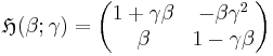
or, if  :
:
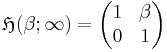
Note that  is not the characteristic constant of f, which is always 1 for a parabolic transformation. From the above expressions one can calculate:

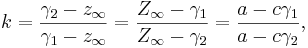
Geometric interpretation of the characteristic constant
The following picture depicts (after stereographic transformation from the sphere to the plane) the two fixed points of a Möbius transformation in the non-parabolic case:
The characteristic constant can be expressed in terms of its logarithm:

When expressed in this way, the real number  becomes an expansion factor. It indicates how repulsive the fixed point is, and how attractive is. The real number is a rotation factor, indicating to what extent the transform rotates the plane anti-clockwise about and clockwise about .
Elliptic transformations
If  , then the fixed points are neither attractive nor repulsive but indifferent, and the transformation is said to be elliptical. These transformations tend to move all points in circles around the two fixed points. If one of the fixed points is at infinity, this is equivalent to doing an affine rotation around a point.
If we take the one-parameter subgroup generated by any elliptic Möbius transformation, we obtain a continuous transformation, such that every transformation in the subgroup fixes the same two points. All other points flow along a family of circles which is nested between the two fixed points on the Riemann sphere. In general, the two fixed points can be any two distinct points.
This has an important physical interpretation. Imagine that some observer rotates with constant angular velocity about some axis. Then we can take the two fixed points to be the North and South poles of the celestial sphere. The appearance of the night sky is now transformed continuously in exactly the manner described by the one-parameter subgroup of elliptic transformations sharing the fixed points  , and with the number corresponding to the constant angular velocity of our observer.
Here are some figures illustrating the effect of an elliptic Möbius transformation on the Riemann sphere (after stereographic projection to the plane):
 |
|
 |
These pictures illustrate the effect of a single Möbius transformation. The one-parameter subgroup which it generates continuously moves points along the family of circular arcs suggested by the pictures.
Hyperbolic transformations
If is zero (or a multiple of  ), then the transformation is said to be hyperbolic. These transformations tend to move points along circular paths from one fixed point toward the other.
If we take the one-parameter subgroup generated by any hyperbolic Möbius transformation, we obtain a continuous transformation, such that every transformation in the subgroup fixes the same two points. All other points flow along a certain family of circular arcs away from the first fixed point and toward the second fixed point. In general, the two fixed points may be any two distinct points on the Riemann sphere.
This too has an important physical interpretation. Imagine that an observer accelerates (with constant magnitude of acceleration) in the direction of the North pole on his celestial sphere. Then the appearance of the night sky is transformed in exactly the manner described by the one-parameter subgroup of hyperbolic transformations sharing the fixed points , with the real number corresponding to the magnitude of his acceleration vector. The stars seem to move along longitudes, away from the South pole toward the North pole. (The longitudes appear as circular arcs under stereographic projection from the sphere to the plane).
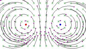
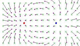
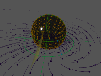
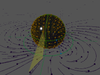
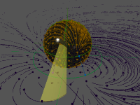
Here are some figures illustrating the effect of a hyperbolic Möbius transformation on the Riemann sphere (after stereographic projection to the plane):
 |
|
 |
These pictures resemble the field lines of bar magnets, because the circular flow lines subtend a constant angle between the two fixed points.
Loxodromic transformations
If both ρ and α are nonzero, then the transformation is said to be loxodromic. These transformations tend to move all points in S-shaped paths from one fixed point to the other.
The word "loxodrome" is from the Greek: "λοξος (loxos), slanting + δρόμος (dromos), course". When sailing on a constant bearing - if you maintain a heading of (say) north-east, you will eventually wind up sailing around the north pole in a logarithmic spiral. On the mercator projection such a course is a straight line, as the north and south poles project to infinity. The angle that the loxodrome subtends relative to the lines of longitude (i.e. its slope, the "tightness" of the spiral) is the argument of k. Of course, Möbius transformations may have their two fixed points anywhere, not just at the north and south poles. But any loxodromic transformation will be conjugate to a transform that moves all points along such loxodromes.
If we take the one-parameter subgroup generated by any loxodromic Möbius transformation, we obtain a continuous transformation, such that every transformation in the subgroup fixes the same two points. All other points flow along a certain family of curves, away from the first fixed point and toward the second fixed point. Unlike the hyperbolic case, these curves are not circular arcs, but certain curves which under stereographic projection from the sphere to the plane appear as spiral curves which twist counterclockwise infinitely often around one fixed point and twist clockwise infinitely often around the other fixed point. In general, the two fixed points may be any two distinct points on the Riemann sphere.
You can probably guess the physical interpretation in the case when the two fixed points are : an observer who is both rotating (with constant angular velocity) about some axis and boosting (with constant magnitude acceleration) along the same axis, will see the appearance of the night sky transform according to the one-parameter subgroup of loxodromic transformations with fixed points , and with  determined respectively by the magnitude of acceleration and angular velocity.
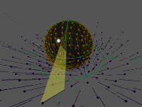
Stereographic projection
These images show Möbius transformations stereographically projected onto the Riemann sphere. Note in particular that when projected onto a sphere, the special case of a fixed point at infinity looks no different from having the fixed points in an arbitrary location.
| Elliptic | Hyperbolic | Loxodromic | |
| One fixed point at infinity |  |
 |
 |
| Full size | Full size | Full size | |
| Fixed points diametrically opposite |  |
 |
 |
| Full size | Full size | Full size | |
| Fixed points in an arbitrary location | 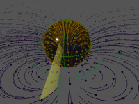 |
 |
 |
| Full size | Full size | Full size |
Iterating a transformation
If a transformation has fixed points , and characteristic constant k, then  will have
  ,
,  ,
,  .
.
This can be used to iterate a transformation, or to animate one by breaking it up into steps.
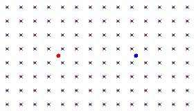
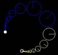
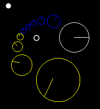
These images show three points (red, blue and black) continuously iterated under transformations with various characteristic constants.
 |
 |
 |
|
And these images demonstrate what happens when you transform a circle under Hyperbolic, Elliptical, and Loxodromic transforms. Note that in the elliptical and loxodromic images, the α value is 1/10 .

Poles of the transformation
The point

is called the pole of ; it is that point which is transformed to the point at infinity under .
The inverse pole

is that point to which the point at infinity is transformed. The point midway between the two poles is always the same as the point midway between the two fixed points:
These four points are the vertices of a parallelogram which is sometimes called the characteristic parallelogram of the transformation.
A transform can be specified with two fixed points and the pole  .
.
This allows us to derive a formula for conversion between  and given :

which reduces down to
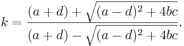
The last expression coincides with one of the (mutually reciprocal) eigenvalue ratios  of the matrix

representing the transform (compare the discussion in the preceding section about the characteristic constant of a transformation). Its characteristic polynomial is equal to

which has roots

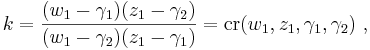
Specifying a transformation by three points
Direct cross-ratio
Fixing three points of a cross-ratio, one obtains a transformation
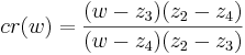
This method allows to directly specify the anti-images of 1, 0, and ∞ respectively as z2, z3, and z4.
The function cr as defined above is obviously a Möbius transformation. It can be easily seen that any Möbius transformation can be written this way. Besides theoretical considerations, it is practical to note that specifying ∞ as one of the zi points cancels out the relevant pair of factors. For example, to get rid of the denominator, that is, to set coefficients c = 0 and d = 1, it is enough to choose ∞ as the anti-image of itself:
Direct approach
Any set of three points

uniquely defines a transformation . To calculate this out, it is handy to make use of a transformation that is able to map three points onto (0,0), (1, 0) and the point at infinity.
One can get rid of the infinities by multiplying out by  and
and  as previously noted.

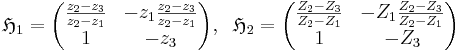
The matrix to map  onto
onto  then becomes

You can multiply this out, if you want, but if you are writing code then it's easier to use temporary variables for the middle terms.
Explicit determinant formula
The problem of constructing a Möbius transformation  mapping a triple
  to another triple
  is equivalent to finding the equation of a standard hyperbola

in the (z,w)-plane passing through the points  . An explicit equation can be found by evaluating the determinant

by means of a Laplace expansion along the first row. This results in the determinant formulae
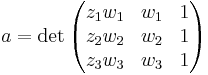
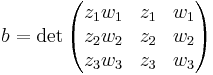
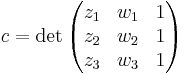
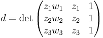
for the coefficients  of the representing matrix
 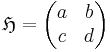 . The constructed matrix has determinant equal to
  which does not vanish if the zi resp. wi are pairwise different thus the Möbius transformation is well-defined.
Remark: A similar determinant (with  replaced by
  ) leads to the equation of a circle through three different (non-collinear) points in the plane.
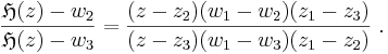
Alternate method using cross-ratios of point quadruples
This construction exploits the fact (mentioned in the first section) that the cross-ratio
is invariant under a Möbius transformation mapping a quadruple  to
to 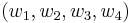 via
via  . If maps a triple of pairwise different zi to another triple , then the
Möbius transformation is determined by the equation

or written out in concrete terms:
The last equation can be transformed into
Solving this equation for one obtains the sought transformation.
Relation to the fixed point normal form
Assume that the points  are the two (different) fixed points of the Möbius transform i.e.
  . Write
 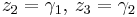 . The last equation
then reads
In the previous section on normal form a Möbius transform with two fixed points was expressed using the characteristic constant k of the transform as
Comparing both expressions one derives the equality
where  is different from the fixed points
  and
and  is the image of z1 under . In particular the cross-ratio
 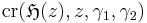 does not depend on the choice of the point z (different from the two fixed points) and is equal to the characteristic constant.
Lorentz transformations
The real Minkowski space consists of a the four-dimensional real coordinate space R4 consisting of the space of ordered quadruples (x0,x1,x2,x3) of real numbers, together with a quadratic form

Borrowing terminology from special relativity, points with Q > 0 are considered timelike; in addition, if x0 > 0, then the point is called future-pointing. Points with Q < 0 are called spacelike. The null cone S consists of those points where Q = 0; the future null cone N+ are those points on the null cone with x0 > 0. The celestial sphere is then identified with the collection of rays in N+ whose initial point is the origin of R4. The collection of linear transformations on R4 with positive determinant preserving the quadratic form Q and preserving the time direction form the orthochronous Lorentz group SO+(1,3).
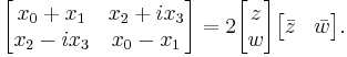
In connection with the geometry of the celestial sphere, the group of transformations SO+(1,3) is identified with the group Möbius transformations of the sphere PSL(2,C) by exhibiting the action of the spin group on spinors (Penrose & Rindler 1986). To each (x0,x1,x2,x3) ∈ R4, associate the hermitian matrix
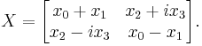
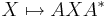
The determinant of the matrix X is equal to Q(x0,x1,x2,x3). The special linear group acts on the space of such matrices via
-
(
for each A ∈ SL(2,C), and this action of SL(2,C) preserves the determinant of X because det A = 1. Since the determinant of X is identified with the quadratic form Q, SL(2,C) acts by Lorentz transformations. On dimensional grounds, SL(2,C) covers a neighborhood of the identity of SO(1,3). Since SL(2,C) is connected, it covers the entire orthochronous Lorentz group SO+(1,3). Furthermore, if is that the kernel of the action (1 ) is the subgroup {±I}, then passing to the quotient group gives the group isomorphism
-

(
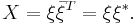
Focussing now attention on the case when (x0,x1,x2,x3) is null, the matrix X has zero determinant, and therefore splits as the outer product of a complex two-vector ξ with its complex conjugate:
-
(
The two-component vector ξ is acted upon by SL(2,C) in a manner compatible with (1 ). It is now clear that the kernel of the representation of SL(2,C) on hermitian matrices is {±I}.
The action of PSL(2,C) on the celestial sphere may also be described geometrically using stereographic projection. Consider first the hyperplane in R4 given by x0 = 1. The celestial sphere may be identified with the sphere S+ of intersection of the hyperplane with the future null cone N+. The stereographic projection from the north pole (1,0,0,1) of this sphere onto the plane x3 = 0 takes a point with coordinates (1,x1,x2,x3) with
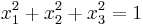
to the point
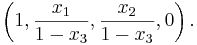
Introducing the complex coordinate
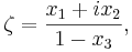
the inverse stereographic projection gives the following formula for a point (x1, x2, x3) on S+:
-

(
The action of SO+(1,3) on the points of N+ does not preserve the hyperplane S+, but acting on points in S+ and then rescaling so that the result is again in S+ gives an action of SO+(1,3) on the sphere which goes over to an action on the complex variable ζ. In fact, this action is by fractional linear transformations, although this is not easily seen from this representation of the celestial sphere. Conversely, for any fractional linear transformation of ζ variable goes over to a unique Lorentz transformation on N+, possibly after a suitable (uniquely determined) rescaling.
A more invariant description of the stereographic projection which allows the action to be more clearly seen is to consider the variable ζ = z:w as a ratio of a pair of homogeneous coordinates for the complex projective line CP1. The stereographic projection goes over to a transformation from C2 − {0} to N+ which is homogeneous of degree two with respect to real scalings
-

(
which agrees with (4 ) upon restriction to scales in which  The components of (5 ) are precisely those obtained from the outer product
In summary, the action of the orthochronous Lorentz group SO+(1,3) agrees with that of the Möbius group PSL(2,C). This motivates the following definition. In dimension n ≥ , the Möbius group Möb(n) is the group of all orientation-preserving conformal isometries of the round sphere Sn to itself. By realizing the conformal sphere as the space of future-pointing rays of the null cone in the Minkowski space R1,n+1, there is an isomorphism of Möb(n) with the orthochronous Lorentz group SO+(1,n+1) of Lorentz transformations with positive determinant, preserving the direction of time.
See also
- Bilinear transform
- Conformal geometry
- Fuchsian group
- Generalised circle
- Hyperbolic geometry
- Inversive geometry
- Inversive ring geometry
- Inversion transformation
- Kleinian group
- Lie sphere geometry
- Lorentz group
- Modular group
- Poincaré half-plane model
- Projective geometry
References
- Beardon, Alan F. (1995), The Geometry of Discrete Groups, New York: Springer-Verlag, ISBN 0-3879-0788-2
- Jones, Gareth A.; Singerman, David (1987), Complex Functions: an Algebraic and Geometric Viewpoint, Cambridge: Cambridge University Press, ISBN 0-521-313666-X (See Chapter 2 for various isomorphisms, and for the Lorentz group viewed as a Galois group.)
- Hall, G. S. (2004), Symmetries and Curvature Structure in General Relativity, Singapore: World Scientific, ISBN 981-02-1051-5 (See Chapter 6 for the classification, up to conjugacy, of the Lie subalgebras of the Lie algebra of the Lorentz group.)
- Katok, Svetlana (1992), Fuchsian Groups, Chicago:University of Chicago Press, ISBN 0-226-42583-5 See Chapter 2.
- Knopp, Konrad (1952), Elements of the Theory of Functions, New York: Dover, ISBN 0-486-60154-4 (See Chapters 3-5 of this classic book for a beautiful introduction to the Riemann sphere, stereographic projection, and Möbius transformations.)
- Mumford, David; Series, Caroline; Wright, David (2002), Indra's Pearls: The Vision of Felix Klein, Cambridge University Press, ISBN 0-521-35253-3 (Aimed at non-mathematicians, provides an excellent exposition of theory and results, richly illustrated with diagrams.)
- Needham, Tristan (1997), Visual Complex Analysis, Oxford: Clarendon Press, ISBN 0-19-853446-9 (See Chapter 3 for a beautifully illustrated introduction to Möbius transformations, including their classification up to conjugacy.)
- Penrose, Roger; Rindler, Wolfgang (1986), Spinors and space-time, Volume 1: Two-spinor calculus and relativistic fields, Cambridge University Press, ISBN 0-521-24527-3
External links
- Eric W. Weisstein, Linear Fractional Transformation at MathWorld.
- Möbius Transformations Revealed, by Douglas N. Arnold and Jonathan Rogness (a video by two University of Minnesota professors explaining and illustrating Möbius transformations using stereographic projection from a sphere). A high resolution version in QuickTime format is available at http://www.ima.umn.edu/~arnold/moebius/index.html .