Matrix (mathematics)

In mathematics, a matrix (plural matrices) is a rectangular table of elements (or entries), which may be numbers or, more generally, any abstract quantities that can be added and multiplied. Matrices are used to describe linear equations, keep track of the coefficients of linear transformations and to record data that depend on multiple parameters. Matrices are described by the field of matrix theory. They can be added, multiplied, and decomposed in various ways, which also makes them a key concept in the field of linear algebra.

Organization of a matrix

Definition

A matrix is a rectangular arrangement of numbers. For example,

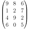
$\begin{bmatrix} 9 & 8 & 6 \\ 1 & 2 & 7 \\ 4 & 9 & 2 \\ 6 & 0 & 5 \end{bmatrix}$ or also denoted using parentheses instead of brackets: $\begin{pmatrix} 9 & 8 & 6 \\ 1 & 2 & 7 \\ 4 & 9 & 2 \\ 6 & 0 & 5 \end{pmatrix}$

is a matrix. The horizontal lines in a matrix are called rows and the vertical lines are called columns. The numbers in the matrix are called its entries. To specify a matrix' size, a matrix with m rows and n columns is called an m-by-n matrix or m × n matrix. m and n are called its dimensions. The dimensions of a matrix are always given with the number of rows first, then the number of columns. It is commonly said that an m-by-n matrix has an order of m × n ("order" meaning size).

A matrix where one of the dimensions equals one is often called a vector, and may be interpreted as an element of real coordinate space. An m × 1 matrix (one column and m rows) is called a column vector and a 1 × n matrix (one row and n columns) is called a row vector. For example, the second row vector of the above matrix is

$\begin{bmatrix} 1 & 2 & 7 \\ \end{bmatrix}$

The entries of a matrix can be rational, real number or complex numbers, or even more general entities.

Notation

The entry that lies in the i-th row and the j-th column of a matrix is typically referred to as the i,j, (i,j), or (i,j)^th entry of the matrix. For example, (2,3) entry of the above matrix is 7.

Matrices are usually denoted using upper-case letters, while the corresponding lower-case letters, with two subscript indices, represent the entries. For example, the (i, j)^th entry of a matrix A is most commonly written as a_i,j. Alternative notations for that entry are A[i,j] or A_i,j. In addition to using upper-case letters to symbolize matrices, many authors use a special typographical style, commonly boldface upright (non-italic), to further distinguish matrices from other variables. Following this convention, A is a matrix, distinguished from A, a scalar. An alternate convention is to annotate matrices with their dimensions in small type underneath the symbol, for example, $\underset{m \times n}{A}$ for an m-by-n matrix.

A common shorthand is

A = (a_i,j)_{i=1,...,m; j=1,...,n} or more briefly A = (a_i,j)_m×n

to define an m × n matrix A. In this case, the entries a_i,j are defined separately for all integers 1 ≤ i ≤ m and 1 ≤ j ≤ n; for example the 2-by-2 matrix

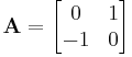
$\mathbf A = \begin{bmatrix} 0 & 1\\ -1 & 0\end{bmatrix}$

is be specified by A = (i − j)_{i=1,2; j=1,2}

In some programming languages the numbering of rows and columns starts at zero, in which case the entries of an m-by-n matrix are indexed by 0 ≤ i ≤ m − 1 and 0 ≤ j ≤ n − 1, but this article will follow the numerotation starting from 1.

Basic operations

There are a number of basic operations that can be applied to modify matrices called matrix addition, (scalar) multiplication and transposition. These, together with the matrix multiplication introduced below are the most important operations related to matrices.

Sum

Main article: Matrix addition

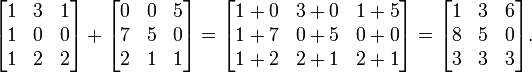
Two or more matrices of identical dimensions m and n can be added. Given m-by-n matrices A and B, their sum A+B is calculated entrywise sum, i.e.

(A + B)_i,j = A_i,j + B_i,j, where 1 ≤ i ≤ m and 1 ≤ j ≤ n.

For example:

$\begin{bmatrix} 1 & 3 & 1 \\ 1 & 0 & 0 \\ 1 & 2 & 2 \end{bmatrix} + \begin{bmatrix} 0 & 0 & 5 \\ 7 & 5 & 0 \\ 2 & 1 & 1 \end{bmatrix} = \begin{bmatrix} 1+0 & 3+0 & 1+5 \\ 1+7 & 0+5 & 0+0 \\ 1+2 & 2+1 & 2+1 \end{bmatrix} = \begin{bmatrix} 1 & 3 & 6 \\ 8 & 5 & 0 \\ 3 & 3 & 3 \end{bmatrix}.$

Another, much less often used notion of matrix addition is the direct sum.

Scalar multiplication

Main article: Scalar multiplication

Given a matrix A and a number (also called a scalar in the parlance of abstract algebra) c, the scalar multiplication cA is computed by multiplying every element of A by c, i.e. (cA)_i,j = c · A_i,j. For example:

$2 \cdot \begin{bmatrix} 1 & 8 & -3 \\ 4 & -2 & 5 \end{bmatrix} = \begin{bmatrix} 2 \cdot 1 & 2\cdot 8 & 2\cdot -3 \\ 2\cdot 4 & 2\cdot -2 & 2\cdot 5 \end{bmatrix} = \begin{bmatrix} 2 & 16 & -6 \\ 8 & -4 & 10 \end{bmatrix}.$

Transpose

Main article: Transpose

The transpose of an m-by-n matrix A is the n-by-m matrix A^T (also denoted by A^tr or ^tA) formed by turning rows into columns and columns into rows, i.e. A^T_i,j = A_j,i.

By inspecting the definition, the following properties of matrix transposition can be derived: (A^T)^T = A, (cA)^T = c(A^T), as well as (A + B)^T = A^T + B^T.

Matrix multiplication and linear transformations

Main article: Matrix multiplication

Multiplication of two matrices is well-defined only if the number of columns of the left matrix is the same as the number of rows of the right matrix. If A is an m-by-n matrix and B is an n-by-p matrix, then their matrix product AB is the m-by-p matrix whose entries are given by

$(\mathbf{AB})_{i,j} = \sum_{r=1}^n A_{i,r}B_{r,j}$

where 1 ≤ i ≤ m and 1 ≤ j ≤ p. For example:

$\begin{align} \begin{bmatrix} 1 & 0 & 2 \\ -1 & 3 & 1 \\ \end{bmatrix} \times \begin{bmatrix} 3 & 1 \\ 2 & 1 \\ 1 & 0 \\ \end{bmatrix} &= \begin{bmatrix} ( 1 \times 3 + 0 \times 2 + 2 \times 1) & ( 1 \times 1 + 0 \times 1 + 2 \times 0) \\ (-1 \times 3 + 3 \times 2 + 1 \times 1) & (-1 \times 1 + 3 \times 1 + 1 \times 0) \end{bmatrix} \\ &= \begin{bmatrix} 5 & 1 \\ 4 & 2 \\ \end{bmatrix}. \end{align}$

Matrix multiplication has the following properties

(AB)C = A(BC) for all k-by-m matrices A, m-by-n matrices B and n-by-p matrices C ("associativity").
(A+B)C = AC+BC for all m-by-n matrices A and B and n-by-k matrices C ("right distributivity").
C(A+B) = CA+CB for all m-by-n matrices A and B and k-by-m matrices C ("left distributivity").

The product AB may be defined without BA being defined, namely if A and B are m-by-n and n-by-k matrices, respectively, and m ≠ k. Even if both products are defined, they need not be equal, i.e. generally one has

AB ≠ BA,

i.e. matrix multiplication is not commutative.

Besides the ordinary matrix multiplication just described, there exist other less frequently used operations on matrices that can be considered forms of multiplication, such as the Hadamard product and the Kronecker product.

Linear transformations

Main articles: Linear transformation and Transformation matrix

Matrices and matrix multiplication reveal their essential features when related to linear transformations (or linear maps). Any n-by-m matrix A gives rise to a linear transformation Rⁿ → R^m, by assigning to any vector x ∈ Rⁿ the (matrix) product Ax, which is an element in R^m. Conversely, given any linear transformation, there exists a matrix A, such that the transformation is given by this formula. The matrix A is said to represent the linear map f, or that A is the transformation matrix of f.

Matrix multiplication neatly corresponds to the composition of maps. If the k-by-m matrix B represents another linear map g : R^m → R^k, then the composition g o f is represented by BA:

$(g \circ f) (\mathbf x) = g (f(\mathbf x)) = g(\mathbf{Ax}) = \mathbf B (\mathbf {Ax}) = (\mathbf {BA}) \mathbf x \,.$

This follows from the above-mentioned associativity of matrix multiplication.

More generally, a linear map from an n-dimensional vector space to an m-dimensional vector space is represented by an m-by-n matrix, provided that bases have been chosen for each. This property makes matrices powerful data structures in high-level programming languages.

Matrix multiplication behaves well with respect to transposition:

(AB)^T = B^TA^T.

If A describes a linear map with respect to two bases, then the matrix A^T describes the transpose of the linear map with respect to the dual bases.

Ranks

Main article: Rank of a matrix

The rank of a matrix A is the dimension of the image of the linear map represented by A; this is the same as the dimension of the space generated by the rows of A, and also the same as the dimension of the space generated by the columns of A. It can also be defined without reference to linear algebra as follows: the rank of an m-by-n matrix A is the smallest number k such that A can be written as a product BC where B is an m-by-k matrix and C is a k-by-n matrix (although this is not a practical way to compute the rank).

Square matrices and related definitions

A square matrix is a matrix which has the same number of rows and columns. The set of all square n-by-n matrices, together with matrix addition and matrix multiplication is a ring. Unless n = 1, this ring is not commutative.

M(n, R), the ring of real square matrices, is a real unitary associative algebra. M(n, C), the ring of complex square matrices, is a complex associative algebra.

The unit matrix or identity matrix I_n of size n is the n-by-n matrix in which all the elements on the main diagonal are equal to 1 and all other elements are equal to 0. The identity matrix is named thus because it satisfies the equations MI_n = M and I_nN = N for any m-by-n matrix M and n-by-k matrix N. For example, if n = 3:

$\mathbf{I}_3 = \begin{bmatrix} 1 & 0 & 0 \\ 0 & 1 & 0 \\ 0 & 0 & 1 \end{bmatrix} .$

The identity matrix is the identity element in the ring of square matrices.

Invertible elements in this ring are called invertible matrices or non-singular matrices. An n-by-n matrix A is invertible if and only if there exists a matrix B such that

AB = I_n ( = BA).

In this case, B is the inverse matrix of A, denoted by A⁻¹. The set of all invertible n-by-n matrices forms a group (specifically a Lie group) under matrix multiplication, the general linear group.

If λ is a number and v is a non-zero vector such that Av = λv, then we call v an eigenvector of A and λ the associated eigenvalue. (Eigen means "own" in German and in Dutch.) The number λ is an eigenvalue of A if and only if A−λI_n is not invertible, which happens if and only if p_A(λ) = 0, where p_A(x) is the characteristic polynomial of A. p_A(x) is a polynomial of degree n and therefore has n complex roots if multiple roots are counted according to their multiplicity. Every square matrix has at most n complex eigenvalues.

The Gaussian elimination algorithm can be used to compute determinants, ranks and inverses of matrices and to solve systems of linear equations.

The trace of a square matrix is the sum of its diagonal entries, which equals the sum of its n eigenvalues.

The square root of a matrix A is any matrix B such that A = B*B, where B* denotes the conjugate transpose of B. The matrix exponential function is defined for square matrices, using power series.

Determinant

The determinant, or the absolute value, in a sense, of a square matrix can be used to solve linear systems and can be found via the application of Cramer's rule. For instance, the linear equation

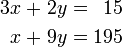
$\begin{alignat}{7} 3x &&\; + \;&& 2y &&\; = \;&& 15 & \\ x &&\; + \;&& 9y &&\; = \;&& 195 & \\ \end{alignat}$

can be solved by finding $x$ and $y$ using matrices and the proper rules:

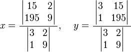
$x=\frac {\,\left| \begin{matrix}15&2\\195&9\end{matrix} \right|\,} {\,\left| \begin{matrix}3&2\\1&9\end{matrix} \right|\,} ,\;\;\;\;y=\frac {\,\left| \begin{matrix}3&15\\1&195\end{matrix} \right|\,} {\,\left| \begin{matrix}3&2\\1&9\end{matrix} \right|\,}$

The operation begins by the finding of the determinants of the matrices; for the 2x2 matrices sampled here, $ad-bc$ is applied to find this particular value. Once the three needed determinants are computed, the fractional equation can be worked out normally. In this instance, $x=-10.2$ and $y=22.8$ . Different and more complex operations are involved for matrices of higher dimension.

Special types of matrices

In many areas in mathematics, matrices with certain structure arise. A few important examples are

Symmetric matrices are such that entries symmetric about the main diagonal (from the upper left to the lower right) are equal, that is, $a_{i,j}=a_{j,i}$ , or equivalently as a matrix equation, $\mathbf{A}^\mathrm{T} = \mathbf{A}$ .
Skew-symmetric matrices are such that entries symmetric about the main diagonal are the negative of each other, that is, $a_{i,j}=-a_{j,i}$ , or equivalently $\mathbf{A}^\mathrm{T}=-\mathbf{A}$ . For obvious reasons all diagonal entries must be zero. No element of the diagonal will be displaced, and therefore each must be its own negative. The only number which satisfies this is zero.
Hermitian (or self-adjoint) matrices are such that entries symmetric about the diagonal are each others complex conjugates, that is, $a_{i,j}=\overline{a}_{j,i}$ , or equivalently $\mathbf{A}^\ast = \mathbf{A}$ , where $\overline{z}$ signifies the complex conjugate of a complex number $z$ and $\mathbf{A}^\ast$ the conjugate transpose of A.
Toeplitz matrices have common entries on all of their diagonals, that is, $A_{i,j}=A_{i+1,j+1}$ .
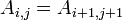Stochastic matrices are square matrices whose rows are probability vectors; they are used to define Markov chains.

For a more extensive list see list of matrices.

Matrices in abstract algebra

If we start with a ring R, we can consider the set M(m,n, R) of all m by n matrices with entries in R. Addition and multiplication of these matrices can be defined as in the case of real or complex matrices (see above). The set M(n, R) of all square n by n matrices over R is a ring in its own right, isomorphic to the endomorphism ring of the left R-module Rⁿ.

Similarly, if the entries are taken from a semiring S, matrix addition and multiplication can still be defined as usual. The set of all square n×n matrices over S is itself a semiring. Note that fast matrix multiplication algorithms such as the Strassen algorithm generally only apply to matrices over rings and will not work for matrices over semirings that are not rings.

If R is a commutative ring, then M(n, R) is a unitary associative algebra over R. It is then also meaningful to define the determinant of square matrices using the Leibniz formula; a matrix is invertible if and only if its determinant is invertible in R.

All statements mentioned in this article for real or complex matrices remain correct for matrices over an arbitrary field.

Matrices over a polynomial ring are important in the study of control theory.

History

The study of matrices is quite old. A 3-by-3 magic square appears in the Chinese literature dating from as early as 650 BC.^[1]

Matrices have a long history of application in solving linear equations. An important Chinese text from between 300 BC and AD 200, The Nine Chapters on the Mathematical Art (Jiu Zhang Suan Shu), is the first example of the use of matrix methods to solve simultaneous equations.^[2] In the seventh chapter, "Too much and not enough," the concept of a determinant first appears almost 2000 years before its publication by the Japanese mathematician Seki Kowa in 1683 and the German mathematician Gottfried Leibniz in 1693.

Magic squares were known to Arab mathematicians, possibly as early as the 7th century, when the Arabs conquered northwestern parts of the Indian subcontinent and learned Indian mathematics and astronomy, including other aspects of combinatorial mathematics. It has also been suggested that the idea came via China. The first magic squares of order 5 and 6 appear in an encyclopedia from Baghdad circa 983 AD, the Encyclopedia of the Brethren of Purity (Rasa'il Ihkwan al-Safa); simpler magic squares were known to several earlier Arab mathematicians.^[1]

The concept of matrix as we know it started with linear algebra. Later, after the development of the theory of determinants by Seki Kowa and Leibniz in the late 17th century, Cramer developed the theory further in the 18th century, presenting Cramer's rule in 1750. Carl Friedrich Gauss and Wilhelm Jordan developed Gauss-Jordan elimination in the 1800s.

The term "matrix" was coined in 1848 by J. J. Sylvester. Cayley, Hamilton, Grassmann, Frobenius and von Neumann are among the famous mathematicians who have worked on matrix theory.

Olga Taussky-Todd (1906-1995) made important contributions to matrix theory, using it to investigate an aerodynamic phenomenon called fluttering or aeroelasticity during World War II. She has been called "a torchbearer" for matrix theory.^[3]

Education

Matrices were traditionally taught as part of linear algebra in college, or with calculus. With the adoption of integrated mathematics texts for use in high school in the United States in the 1990s, they have been included by many such texts such as the Core-Plus Mathematics Project which are often targeted as early as the ninth grade, or earlier for honors students. They often require the use of graphing calculators which can perform complex operations such as matrix inversion very quickly.

Although most computer languages are not designed with commands or libraries for matrices, as early as the 1970s, some engineering desktop computers such as the HP 9830 had ROM cartridges to add BASIC commands for matrices. Some computer languages such as APL, were designed to manipulate matrices, and mathematical programs such as Mathematica, and others are used to aid computing with matrices.

Applications

Encryption

See also: Hill cipher

Matrices can be used to encrypt numerical data. Encryption is done by multiplying the data matrix with a key matrix. Decryption is done simply by multiplying the encrypted matrix with the inverse of the key.

Computer graphics

See also: Transformation matrix

4×4 transformation affine rotation matrices are commonly used in computer graphics. The upper left 3×3 portion of a transformation matrix is composed of the new X, Y, and Z axes of the post-transformation coordinate space.

References

↑ ^1.0 ^1.1 Swaney, Mark. History of Magic Squares.
↑ Shen Kangshen et al. (ed.) (1999). Nine Chapters of the Mathematical Art, Companion and Commentary. Oxford University Press. cited by Otto Bretscher (2005). Linear Algebra with Applications (3rd ed. ed.). Prentice-Hall. pp. p. 1.
↑ Ivars Peterson. Matrices, Circles, and Eigenthings.

External links

Resources
- Matrix name and history: very brief overview, ualr.edu
- Introduction to Matrix Algebra: definitions and properties, xycoon.com
- Matrix Algebra, sosmath.com
- The Matrix Reference Manual, Imperial College
- The Matrix Cookbook, A free mathematical desktop reference on matrices
- Applied examples of matrices used in graphical game programming, Riemer's DirectX Tutorials
- An Introduction to Matrix Algebra by Autar Kaw, A simple primer for a beginner or one who is rusty on the topic

Online Matrix Calculators
- easycalculation.com
- Matri-tri-ca - Matrix Calculator
- bluebit.gr
- wims.unice.fr
- Matrix Calculator at SolveMyMath - Calculate the Determinant, Trace, Transpose and Inverse Matrix of a Matrix

Freeware
- MATRIX 2.1 Excel add-in, foxes
- MacAnova, University of Minnesota School of Statistics