Limit of a function

x	$\frac{\sin x}{x}$
1	0.841471
0.1	0.998334
0.01	0.999983

Although the function (sin x)/x is not defined at zero, as x becomes closer and closer to zero, (sin x)/x becomes arbitrarily close to 1. We say that "the limit of (sin x)/x as x approaches zero equals 1."

Topics in calculus
Fundamental theorem Limits of functions Continuity Vector calculus Matrix calculus Mean value theorem
Differentiation
Product rule Quotient rule Chain rule Change of variables Implicit differentiation Taylor's theorem Related rates List of differentiation identities
Integration
Lists of integrals Improper integrals Integration by: parts, disks, cylindrical shells, substitution, trigonometric substitution, partial fractions, changing order

In mathematics, the limit of a function is a fundamental concept in calculus and analysis concerning the behavior of that function near a particular input. Informally, a function assigns an output f(x) to every input x. The function has a limit L at an input p if f(x) is "close" to L whenever x is "close" to p. In other words, f(x) becomes closer and closer to L as x moves closer and closer to p. More specifically, when f is applied to each input sufficiently close to p, the result is an output value that is arbitrarily close to L. If the inputs "close" to p are taken to values that are very different, the limit is said to not exist. Formal definitions, first devised in the early 19th century, are given below.

1 History
2 Motivation
3 Definitions
4 Example
5 Properties
6 See also
7 References

History

Although implicit in the development of Calculus of the 17th and 18th centuries, the modern notion of the limit of a function goes back to Bolzano who, in 1817, introduced the basics of the epsilon-delta technique.^[1] However, his work was not known during his lifetime. Cauchy discussed limits in his Cours d'analyse (1821) and seems to have expressed the essence of the idea, but not in a systematic fashion.^[2] The first rigorous public presentation of the technique was given by Weierstrass in the 1850s and 1860s^[3] and has since become the standard method for dealing with limits.

The written notation using the lim abbreviation together with the arrow below is due to Hardy in his book A Course of Pure Mathematics in 1908.^[2]

Motivation

Imagine a person walking over a landscape represented by the graph of y = f(x). Her horizontal position is measured by the value of x, much like the position given by a map of the land or by a global positioning system. Her altitude is given by the coordinate y. She is walking towards the horizontal position given by x = p. As she does so, she notices that her altitude approaches L. If later asked to guess the altitude over x = p, she would then answer L, even if she had never actually reached that position.

What, then, does it mean to say that her altitude approaches L? It means that her altitude gets nearer and nearer to L except for a possible small error in accuracy. For example, suppose we set a particular accuracy goal for our traveler: she must get within ten meters of L. She reports back that indeed she can get within ten meters of L, since she notes that when she is within fifty horizontal meters of p, her altitude is always ten meters or less from L.

We then change our accuracy goal: can she get within one meter? Yes. If she is within seven horizontal meters of p, then her altitude remains within one meter of the target L. In summary, to say that the traveler's altitude approaches L as her horizontal position approaches p means that for every target accuracy goal, there is some neighborhood of p whose altitude remains within that accuracy goal.

The initial informal statement can now be explicated:

The limit of a function f(x) as x approaches p is a number L with the following property: given any target distance from L, there is a distance from p within which the values of f(x) remain within the target distance.

This explicit statement is quite close to the formal definition of the limit of a function with values in a topological space.

Definitions

The following definitions (known as (ε, δ)-definitions) are the generally accepted ones for the limit of a function in various contexts.

Functions on the real line

Suppose f : R → R is defined on the real line and p,L ∈ R then we say the limit of f as x approaches p is L and write

$\lim_{x \to p}f(x) = L$

if and only if for every real ε > 0 there exists a real δ > 0 such that 0 < | x - p | < δ implies | f(x) - L | < ε. Note that the value of the limit does not depend on the value of f(p).

A more general definition applies for functions defined on subsets of the real line. Let (a,b) be an open interval in R, and p a point of (a,b). Let f be a real-valued function defined on all of (a, b) except possibly at p. We then say that the limit of f as x approaches p is L if and only if, for every real ε > 0 there exists a real δ > 0 such that 0 < | x - p | < δ and x ∈ (a,b) implies | f(x) - L | < ε. Note that the limit does not depend on f(p) being well-defined.

One-sided limits

Main article: One-sided limit

The limit as: x → x₀⁺ ≠ x → x₀^-. Therefore, the limit as x → x₀ does not exist.

Alternatively x may approach p from above (right) or below (left), in which case the limits may be written as

$\lim_{x \to p^+}f(x) = L$

$\lim_{x \to p^-}f(x) = L$

respectively. If both of these limits are equal to L then this can be referred to as the limit of f(x) at p. Conversely, if they are not both equal to L then the limit, as such, does not exist.

A formal definition is as follows. The limit of f(x) as x approaches p from above is L if, for every ε > 0, there exists a δ > 0 such that |f(x) - L| < ε whenever 0 < x - p < δ. The limit of f(x) as x approaches p from below is L if, for every ε > 0, there exists a δ > 0 such that |f(x) - L| < ε whenever 0 < p - x < δ.

If the limit does not exist there is a non-zero oscillation.

Functions on metric spaces

Suppose f : (M,d_M) → (N,d_N) is defined between two metric spaces, with x ∈ M, p a limit point of M and L ∈ N. We say that the limit of f as x approaches p is L and write

$\lim_{x \to p}f(x) = L$

if and only if for every ε > 0 there exists a δ > 0 such that, d_N(f(x), L) < ε whenever 0 < d_M(x, p) < δ. Again, note that p need not be in the domain of f, nor does L need to be in the range of f.

An alternative definition using the concept of neighbourhood is as follows:

$\lim_{x \to p}f(x) = L$

if and only if for every neighbourhood V of L in N there exists a neighbourhood U of p in M, such that f(U - {p}) ⊆ V.

Functions on topological spaces

Suppose X,Y are topological spaces with Y a Hausdorff space. Let p be a limit point of X, and L ∈Y. For a function f : X-{p} → Y, we say that the limit of f as x approaches p is L (i.e., f(x)→L as x→p) and write

$\lim_{x \to p}f(x) = L$

if and only if for every neighborhood V of L, there exists a neighborhood U of p such that f(U- {p}) ⊆ V.

Note that the domain of f does not need to contain p. If it does, then the value of f at p is irrelevant to the definition of the limit. The last part of the definition can also be phrased "there exists a punctured neighbourhood U of p such that f(U) ⊆ V ".

One can formulate other similar definitions of the limit in a topological space. In one version, the domain of the function f is a subset Ω of the topological space X. In this case, the point p must be a limit point of Ω, and the limit is taken with respect to the induced topology on Ω (one-sided limits, where the limit is taken inside an interval at one of the endpoints, are a special case of this).

In particular, if the domain of f is X - {p} (or all of X), then the limit of f as x → p exists and is equal to L if and only if for all subsets Ω of X with limit point p the limit of the restriction of f to Ω exists and is equal to L. Sometimes this criterion is used to establish the non-existence of the two-sided limit of a function on R by showing that the one-sided limits either fail to exist or do not agree. Such a view is fundamental in the field of general topology, where limits and continuity at a point are defined in terms of special families of subsets, called filters, or generalized sequences known as nets.

Alternatively, the requirement that Y be a Hausdorff space can be relaxed to the assumption that Y be a general topological space, but then the limit of a function will not be unique. In particular, one can no longer talk about the limit of a function at a point, but rather a limit or the set of limits at a point.

A function is continuous in a limit point p of and in its domain if and only f(p) is the (or, in the general case, a) limit of f(x) as x tends to p.

Limit of a function at infinity

The limit of this function at infinity exists.

If the extended real line R is considered, i.e., R ∪ {-∞, +∞}, then it is possible to define limits of a function at infinity.

If f(x) is a real function, then the limit of f as x approaches infinity is L, denoted

$\lim_{x \to \infty}f(x) = L,$

if and only if for all $\epsilon > 0$ there exists S > 0 such that $|f(x) - L| < \epsilon$ whenever x > S.

Similarly, the limit of f as x approaches infinity is infinity, denoted

$\lim_{x \to \infty}f(x) = \infty,$

if and only if for all R > 0 there exists S > 0 such that f(x) > R whenever x > S.

In an analogous way, the following expressions can be defined:

$\lim_{x \to -\infty}f(x) = L, \lim_{x \to \infty}f(x) = -\infty, \lim_{x \to -\infty}f(x) = \infty, \lim_{x \to -\infty}f(x) = -\infty$ .

These notions of a limit attempt to provide a metric space interpretation to limits at infinity. However, note that these notions of a limit are consistent with the topological space definition of limit if

a neighborhood of -∞ is defined to contain an interval [-∞,c) where c∈R
a neighborhood of ∞ is defined to contain an interval (c,∞] where c∈R
a neighborhood of a∈R is defined in the normal way metric space R

In this case, R is a topological space and any function of the form f:X → Y with X,Y⊆ R is subject to the topological definition of a limit. Note that with this topological definition, it is easy to define infinite limits at finite points, which have not been defined above in the metric sense.

Evaluating limits at infinity for rational functions

Horizontal Asymptote about y= 4

There are three basic rules for evaluating limits at infinity for a rational function f(x) = p(x)/q(x):

If the degree of p is greater than the degree of q, then the limit is positive or negative infinity depending on the signs of the leading coefficients;
If the degree of p and q are equal, the limit is the leading coefficient of p divided by the leading coefficient of q;
If the degree of p is less than the degree of q, the limit is 0.

If the limit at infinity exists, it represents a horizontal asymptote at y = L. Polynomials do not have horizontal asymptotes; they may occur with rational functions.

Complex-valued functions

The complex plane with metric 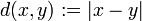$d(x, y)�:= |x-y|$ is also a metric space. There are two different types of limits when we consider complex-valued functions.

Limit of a function at a point

If f is a complex-valued function, then

$\lim_{x \to p} f(x) = L$

if and only if for all ε > 0 there exists a δ > 0 such that for all real numbers x with $0 < |x - p| < \delta$ , we have $|f(x) - L| < \epsilon$ .

It is just a particular case of functions over metric spaces with both M and N are the complex plane.

Limit of a function of more than one variable

By noting that |x-p| represents a distance, the definition of a limit can be extended to functions of more than one variable. In the case of a function f : R² → R,

$\lim_{(x,y) \to (p, q)} f(x, y) = L$

if and only if

for every ε > 0 there exists a δ > 0 such that for all (x,y) with 0 < ||(x,y)-(p,q)|| < δ, we have |f(x,y)-L| < ε

where ||(x,y)-(p,q)|| represents the Euclidean distance. This can be extended to any number of variables.

Sequential limits

Let f : X → Y be a mapping from a topological space X into a Hausdorff space Y, p∈X and L∈Y.

The sequential limit of f as x→p is L if and only if, for every sequence (x_n) in X which converges to p, the sequence f(x_n) converges to L.

If L is the limit (in the sense above) of f as x approaches p, then it is a sequential limit as well, however the converse need not hold in general. If in addition Y is metrizable, then L is the sequential limit of f as x approaches p if and only if it is the limit (in the sense above) of f as x approaches p.

Example

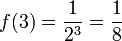
Take the function $f(x)=\frac{1}{2^x}$ where $x$ is a non-negative integer. When x is systematically substituted by consecutive values along the natural line, we see a pattern emerging:

$f(0)=\frac{1}{2^0}=\frac{1}{1}=1$

$f(1)=\frac{1}{2^1}=\frac{1}{2}$

$f(2)=\frac{1}{2^2}=\frac{1}{4}$

$f(3)=\frac{1}{2^3}=\frac{1}{8}$

$f(4)=\frac{1}{2^4}=\frac{1}{16}$

When $x$ is substituted with a significantly large value, we begin to see that f(x) ≈ 0:

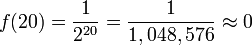
$f(20)=\frac{1}{2^{20}}=\frac{1}{1,048,576}\approx0$

$f(50)=\frac{1}{2^{50}}\approx0$

As x becomes larger, f(x) approaches 0. This is denoted : $\lim_{x \to \infty}f(x) = 0$

Properties

If the sets A, B, ... form a finite partition of the function domain, $x\in\overline{A} \land x\in\overline{B}$ , ... and the relative limit for each of those sets exist and is the equal to, say, L, then the limit exists for the point x and is equal to L. In particular, if f is real-valued, then the limit of f at p is L if and only if both the right-handed limit and left-handed limit of f at p exist and are equal to L.

The function f is continuous at p if and only if the limit of f(x) as x approaches p exists and is equal to f(p). If f : M → N is a function between metric spaces M and N, then it is equivalent that f transforms every sequence in M which converges towards p into a sequence in N which converges towards f(p).

If N is a normed vector space, then the limit operation is linear in the following sense: if the limit of f(x) as x approaches p is L and the limit of g(x) as x approaches p is P, then the limit of f(x) + g(x) as x approaches p is L + P. If a is a scalar from the base field, then the limit of af(x) as x approaches p is aL.

If f is a real-valued (or complex-valued) function, then taking the limit is compatible with the algebraic operations, provided the limits on the right sides of the identity below exist:

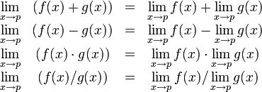
$\begin{matrix} \lim\limits_{x \to p} & (f(x) + g(x)) & = & \lim\limits_{x \to p} f(x) + \lim\limits_{x \to p} g(x) \\ \lim\limits_{x \to p} & (f(x) - g(x)) & = & \lim\limits_{x \to p} f(x) - \lim\limits_{x \to p} g(x) \\ \lim\limits_{x \to p} & (f(x)\cdot g(x)) & = & \lim\limits_{x \to p} f(x) \cdot \lim\limits_{x \to p} g(x) \\ \lim\limits_{x \to p} & (f(x)/g(x)) & = & {\lim\limits_{x \to p} f(x) / \lim\limits_{x \to p} g(x)} \end{matrix}$

(the last provided that the denominator is non-zero). In each case above, when the limits on the right do not exist, or, in the last case, when the limits in both the numerator and the denominator are zero, nonetheless the limit on the left, called an indeterminate form, may still exist — this depends on the functions f and g. These rules are also valid for one-sided limits, for the case p = ±∞, and also for infinite limits using the rules

q + ∞ = ∞ for q ≠ -∞
q × ∞ = ∞ if q > 0
q × ∞ = −∞ if q < 0
q / ∞ = 0 if q ≠ ± ∞

(see extended real number line).

Note that there is no general rule for the case q / 0; it all depends on the way 0 is approached. Indeterminate forms — for instance, 0/0, 0×∞, ∞−∞, and ∞/∞ — are also not covered by these rules, but the corresponding limits can often be determined with L'Hôpital's rule or the Squeeze theorem.

References

Visual Calculus by Lawrence S. Husch, University of Tennessee (2001)

Apostol, Tom M., Mathematical Analysis, 2nd ed. Addison-Wesley, 1974. ISBN 0201002884.

Sutherland, W. A., Introduction to Metric and Topological Spaces. Oxford University Press, Oxford, 1975. ISBN 0 19 853161 3.

Limit of a function

Contents

History

Motivation

Definitions

Functions on the real line

One-sided limits

Functions on metric spaces

Functions on topological spaces

Limit of a function at infinity

Evaluating limits at infinity for rational functions

Complex-valued functions

Limit of a function at a point

Limit of a function of more than one variable

Sequential limits

Example

Properties

See also

References