Law of large numbers

A demonstration of the Law of Large Numbers using die rolls.

The law of large numbers (LLN) is a theorem in probability that describes the long-term stability of the mean of a random variable. Given a random variable with a finite expected value, if its values are repeatedly sampled, as the number of these observations increases, their mean will tend to approach and stay close to the expected value.

The LLN can easily be illustrated using the rolls of a die. That is, outcomes of a multinomial distribution in which the numbers 1, 2, 3, 4, 5, and 6 are equally likely to be chosen. The population mean (or "expected value") of the outcomes is:

(1 + 2 + 3 + 4 + 5 + 6) / 6 = 3.5.

The graph to the right plots the results of an experiment of rolls of a die. In this experiment we see that the average of die rolls deviates wildly at first. As predicted by LLN the average stabilizes around the expected value of 3.5 as the number of observations becomes large.

Another example is the flip of a coin. Given repeated flips of a fair coin, the frequency of heads (or tails) will increasingly approach 50% over a large number of trials. However it is possible that the absolute difference in the number of heads and tails will tend to get larger and larger as the number of flips increases.^[1] For example, we may see 520 heads after 1000 flips and 5096 heads after 10000 flips. While the average has moved from 0.52 to 0.5096, closer to the expected 50%, the total difference from the expected mean has increased from 20 to 96.

The LLN is important because it "guarantees" stable long-term results for random events. For example, while a casino may lose money in a single spin of the roulette wheel, its earnings will tend towards a predictable percentage over a large number of spins. Any winning streak by a player will eventually be overcome by the parameters of the game. It is important to remember that the LLN only applies (as the name indicates) when a large number of observations are considered. There is no principle that a small number of observations will converge to the expected value or that a streak of one value will immediately be "balanced" by the others. See the Gambler's fallacy.

1 History
2 Forms
3 Activities and demonstrations
4 See also
5 References
6 External links

History

The LLN was first described by Jacob Bernoulli.^[2] It took him over 20 years to develop a sufficiently rigorous mathematical proof which was published in his Ars Conjectandi (The Art of Conjecturing) in 1713. He named this his "Golden Theorem" but it became generally known as "Bernoulli's Theorem" (not to be confused with the Law in Physics with the same name.) In 1835, S.D. Poisson further described it under the name "La loi des grands nombres" ("The law of large numbers").^[3] Thereafter, it was known under both names, but the "Law of large numbers" is most frequently used.

After Bernoulli and Poisson published their efforts, other mathematicians also contributed to refinement of the law, including Chebyshev, Markov, Borel, Cantelli and Kolmogorov. These further studies have given rise to two prominent forms of the LLN. One is called the "weak" law and the other the "strong" law. These forms do not describe different laws but instead refer to different ways of describing the mode of convergence of the cumulative sample means to the expected value, and the strong form implies the weak.

Forms

Both versions of the law state that the sample average

$\overline{X}_n=\frac1n(X_1+\cdots+X_n)$

converges to the expected value

$\overline{X}_n \, \to \, \mu \qquad\textrm{for}\qquad n \to \infty$

where X₁, X₂, ... is an infinite sequence of i.i.d. random variables with finite expected value E(X₁) = E(X₂) = ... = µ < ∞.

An assumption of finite variance Var(X₁) = Var(X₂) = ... = σ² < ∞ is not necessary. Large or infinite variance will make the convergence slower, but the LLN holds anyway. This assumption is often used because it makes the proofs easier and shorter.

The difference between the strong and the weak version is concerned with the mode of convergence being asserted.

The weak law

The weak law of large numbers states that the sample average converges in probability towards the expected value

$\overline{X}_n \, \xrightarrow{P} \, \mu \qquad\textrm{for}\qquad n \to \infty.$

That is to say that for any positive number ε,

$\lim_{n\rightarrow\infty}\operatorname{P}\left(\left|\overline{X}_n-\mu\right|<\varepsilon\right)=1.$

(Proof)

Interpreting this result, the weak law essentially states that for any nonzero margin specified, no matter how small, with a sufficiently large sample there will be a very high probability that the average of the observations will be close to the expected value, that is, within the margin.

Convergence in probability is also called weak convergence of random variables. This version is called the weak law because random variables may converge weakly (in probability) as above without converging strongly (almost surely) as below.

A consequence of the weak LLN is the asymptotic equipartition property.

The strong law

The strong law of large numbers states that the sample average converges almost surely to the expected value

$\overline{X}_n \, \xrightarrow{\mathrm{a.s.}} \, \mu \qquad\textrm{for}\qquad n \to \infty .$

That is,

$\operatorname{P}\left(\lim_{n\rightarrow\infty}\overline{X}_n=\mu\right)=1,$

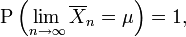
The proof is more complex than that of the weak law. This law justifies the intuitive interpretation of the expected value of a random variable as the "long-term average when sampling repeatedly."

Almost sure convergence is also called strong convergence of random variables. This version is called the strong law because random variables which converge strongly (almost surely) are guaranteed to converge weakly (in probability). The strong law implies the weak law.

The strong law of large numbers can itself be seen as a special case of the ergodic theorem.

Differences between the weak law and the strong law

The Weak Law states that, for a specified large $n$ , $(X_1+...+X_n)/n$ is likely to be near $\mu$ . Thus, it leaves open the possibility that $(X_1+...+X_n)/n -\mu$ happens an infinite number of times, although it happens at infrequent intervals.

The strong law shows that this cannot occur. In particular, it implies that with probability 1, for any positive value $\epsilon$ , $(X_1+...+X_n)/n-\mu$ will be greater than $\epsilon$ only a finite number of times. ^[4]

Activities and demonstrations

There are varieties of ways to illustrate the theory and applications of the laws of large numbers using interactive aids. The SOCR resource provides a hands-on learning activity paired with a Java applet (select the Coin Toss LLN Experiment) that demonstrate the power and usability of the law of large numbers.

References

↑ Tijms, Henk (2007). Understanding Probability: Chance Rules in Everyday Life. Cambridge University Press. pp. 17. ISBN 978-0-521-70172-3. http://books.google.com/books?id=Ua-_5Ga4QF8C&printsec=frontcover#PRA2-PA17,M1.
↑ Jakob Bernoulli, Ars Conjectandi: Usum & Applicationem Praecedentis Doctrinae in Civilibus, Moralibus & Oeconomicis, 1713, Chapter 4, (Translated into English by Oscar Sheynin)
↑ Hacking, Ian. (1983) "19th-century Cracks in the Concept of Determinism"
↑ Sheldon Ross, A First Course in Probability, Fifth edition, Prentice Hall press

Grimmett, G. R. and Stirzaker, D. R. (1992). Probability and Random Processes, 2nd Edition. Clarendon Press, Oxford. ISBN 0-19-853665-8.
Richard Durrett (1995). Probability: Theory and Examples, 2nd Edition. Duxbury Press.
Martin Jacobsen (1992). Videregående Sandsynlighedsregning (Advanced Probability Theory) 3rd Edition''. HCØ-tryk, Copenhagen. ISBN 87-91180-71-6.

External links

MathWorld: Weak Law of Large Numbers
MathWorld: Strong Law of Large Numbers
Animations for the Law of Large Numbers by Yihui Xie using the R package animation

Large numbers

Subarticles

Names of large numbers · Law of large numbers · History of large numbers

Examples (numerical order)
Standardized list · Name list

million · billion · trillion · quadrillion · googol · googolplex · Skewes' number · Moser's number · Graham's number · Transfinite numbers · Infinity

Expression methods

Notations	Steinhaus-Moser notation · Knuth's up-arrow notation · Conway chained arrow notation

Operators	Hyper operators · Ackermann function · Tetration

Number systems · Number names · Orders of magnitude (numbers) · List of numbers · Indefinite and fictitious numbers