Lagrange multipliers

 subject to a constraint (shown in red)
  .
. . The blue lines are contours of . The intersection of red and blue lines is our solution.
In mathematical optimization, the method of Lagrange multipliers (named after Joseph Louis Lagrange) is a method for finding the maximum/minimum of a function subject to constraints.
For example (see Figure 1 on the right) if we want to solve:
- maximize

- subject to

We introduce a new variable ( ) called a Lagrange multiplier to rewrite the problem as:
- maximize
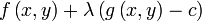
Solving this new unconstrained problem for x, y, and will give us the solution (x, y) for our original constrained problem.
Contents |
Introduction
Consider a two-dimensional case. Suppose we have a function we wish to maximize or minimize subject to the constraint

where c is a constant. We can visualize contours of  given by
for various values of  , and the contour of
  given by .
Suppose we walk along the contour line with  . In general the contour lines of and may be distinct, so traversing the contour line for could intersect with or cross the contour lines of . This is equivalent to saying that while moving along the contour line for the value of can vary. Only when the contour line for touches contour lines of tangentially, we do not increase or decrease the value of - that is, when the contour lines touch but do not cross.
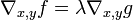
This occurs exactly when the tangential component of the total derivative vanishes:  , which is at the constrained stationary points of (which include the constrained local extrema, assuming is differentiable). Computationally, this is when the gradient of is normal to the constraint(s): when
  for some scalar (where
  is the gradient). Note that the constant is required because, even though the directions of both gradient vectors are equal, the magnitudes of the gradient vectors are generally not equal.
A familiar example can be obtained from weather maps, with their contour lines for temperature and pressure: the constrained extrema will occur where the superposed maps show touching lines (isopleths).
Geometrically we translate the tangency condition to saying that the gradients of and are parallel vectors at the maximum, since the gradients are always normal to the contour lines. Thus we want points  where and
 ,
,
where
To incorporate these conditions into one equation, we introduce an auxiliary function

and solve
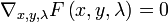 .
.
Justification
As discussed above, we are looking for stationary points of seen while travelling on the level set . This occurs just when the gradient of has no component tangential to the level sets of . This condition is equivalent to  for some . Stationary points
  of
of  also satisfy as can be seen by considering the derivative with respect to . In other words, taking the derivative of the auxillary function with respect to and setting it equal to zero is the same thing as taking the constraint equation into account.
Caveat: extrema versus stationary points
Be aware that the solutions are the stationary points of the Lagrangian , and may be saddle points: they are not necessarily extrema of . is unbounded: given a point that doesn't lie on the constraint, letting  makes arbitrarily large or small. However, under certain stronger assumptions, as we shall see below, the strong Lagrangian principle holds, which states that the maxima of maximize the Lagrangian globally.
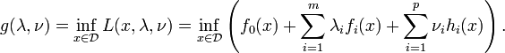
A more general formulation: The weak Lagrangian principle
Denote the objective function by  and let the constraints be given by
  . The domain of f should be an open set containing all points satisfying the constraints. Furthermore, and the
  must have continuous first partial derivatives and the gradients of the must not be zero on the domain.[1] Now, define the Lagrangian,
  , as
, as
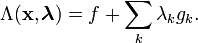
 is an index for variables and functions associated with a particular constraint, .
 without a subscript indicates the vector with elements
  , which are taken to be independent variables.
Observe that both the optimization criteria and constraints  are compactly encoded as stationary points of the Lagrangian:
 if and only if
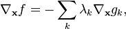
 means to take the gradient only with respect to each element in the vector
  , instead of all variables.
and
 implies
Collectively, the stationary points of the Lagrangian,
 ,
,
give a number of unique equations totaling the length of plus the length of  .
.
Interpretation of 
Often the Lagrange multipliers have an interpretation as some salient quantity of interest. To see why this might be the case, observe that:

So, λk is the rate of change of the quantity being optimized as a function of the constraint variable. As examples, in Lagrangian mechanics the equations of motion are derived by finding stationary points of the action, the time integral of the difference between kinetic and potential energy. Thus, the force on a particle due to a scalar potential,  , can be interpreted as a Lagrange multiplier determining the change in action (transfer of potential to kinetic energy) following a variation in the particle's constrained trajectory. In economics, the optimal profit to a player is calculated subject to a constrained space of actions, where a Lagrange multiplier is the value of relaxing a given constraint (e.g. through bribery or other means).
The method of Lagrange multipliers is generalized by the Karush-Kuhn-Tucker conditions.
Examples
Very simple example

Suppose you wish to maximize 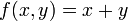 subject to the constraint
  . The constraint is the unit circle, and the level sets of f are diagonal lines (with slope -1), so one can see graphically that the maximum occurs at
  (and the minimum occurs at
Formally, set  , and
, and

Set the derivative  , which yields the system of equations:
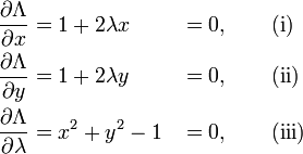
As always, the  equation is the original constraint.
Combining the first two equations yields  (explicitly,
  ,otherwise (i) yields 1 = 0), so one can solve for , yielding
 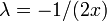 , which one can substitute into (ii)).
Substituting into (iii) yields  , so
, so  and the stationary points are and . Evaluating the objective function f on these yields

thus the maximum is  , which is attained at and the minimum is
  , which is attained at .
Simple example
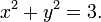
Suppose you want to find the maximum values for
with the condition that the x and y coordinates lie on the circle around the origin with radius √3, that is,
As there is just a single condition, we will use only one multiplier, say λ.
Use the constraint to define a function g(x, y):
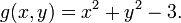
The function g is identically zero on the circle of radius √3. So any multiple of g(x, y) may be added to f(x, y) leaving f(x, y) unchanged in the region of interest (above the circle where our original constraint is satisfied). Let

The critical values of occur when its gradient is zero. The partial derivatives are
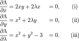
Equation (iii) is just the original constraint. Equation (i) implies  or λ = −y. In the first case, if then we must have
  by (iii) and then by (ii) λ=0. In the second case, if λ = −y and substituting into equation (ii) we have that,
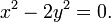
Then x2 = 2y2. Substituting into equation (iii) and solving for y gives this value of y:

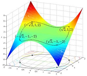
Thus there are six critical points:

Evaluating the objective at these points, we find

Therefore, the objective function attains a global maximum (with respect to the constraints) at  and a global minimum at
  The point
  is a local minimum and
  is a local maximum.
Example: entropy
Suppose we wish to find the discrete probability distribution with maximal information entropy. Then
Of course, the sum of these probabilities equals 1, so our constraint is g(p) = 1 with
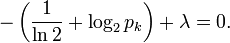
We can use Lagrange multipliers to find the point of maximum entropy (depending on the probabilities). For all k from 1 to n, we require that
which gives
Carrying out the differentiation of these n equations, we get
This shows that all pi are equal (because they depend on λ only). By using the constraint ∑k pk = 1, we find

Hence, the uniform distribution is the distribution with the greatest entropy.
Economics
Constrained optimization plays a central role in economics. For example, the choice problem for a consumer is represented as one of maximizing a utility function subject to a budget constraint. The Lagrange multiplier has an economic interpretation as the shadow price associated with the constraint, in this case the marginal utility of income.
The strong Lagrangian principle: Lagrange duality
Given a convex optimization problem in standard form
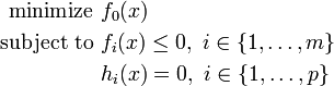
with the domain  having non-empty interior, the Lagrangian function
  is defined as
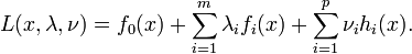
The vectors and  are called the dual variables or Lagrange multiplier vectors associated with the problem. The Lagrange dual function
  is defined as
The dual function is concave, even when the initial problem is not convex. The dual function yields lower bounds on the optimal value  of the initial problem; for any
  and any we have
 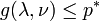 . If a constraint qualification such as Slater's condition holds and the original problem is convex, then we have strong duality, i.e.
 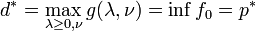 .
.
See also
- Karush-Kuhn-Tucker conditions: generalization of the method of Lagrange multipliers.
- Lagrange multipliers on Banach spaces: another generalization of the method of Lagrange multipliers.
References
- ↑ Gluss, David and Weisstein, Eric W., Lagrange Multiplier at MathWorld.
External links
Exposition
- Conceptual introduction (plus a brief discussion of Lagrange multipliers in the calculus of variations as used in physics)
- Lagrange Multipliers without Permanent Scarring (tutorial by Dan Klein)
For additional text and interactive applets