Labour economics
| Economics |
| Outline of topics |
|---|
| General classifications |
|
Microeconomics · Macroeconomics |
| Techniques |
|
Mathematical · Econometrics |
| Fields and subfields |
|
Behavioral · Cultural · Evolutionary |
| Lists |
|
Journals · Publications |
Labour economics seeks to understand the functioning of the market and dynamics for labour. Labour markets function through the interaction of workers and employers. Labour economics looks at the suppliers of labour services (workers), the demanders of labour services (employers), and attempts to understand the resulting pattern of wages, employment, and income.
It is an important subject because unemployment is a problem that affects the public most directly and severely. Full employment (or reduced unemployment) is a goal of many modern governments. Other often studied markets are financial market and product market.
In economics, labour (or labor) is a measure of the work done by human beings. It is conventionally contrasted with such other factors of production as land and capital. There are theories which have created a concept called human capital (referring to the skills that workers possess, not necessarily their actual work), although there are also counter posing macro-economic system theories that think human capital is a contradiction in terms.
Compensation and measurement
| [hide]Part of a series on
Organized labour |
|---|
 |
| The labour movement |
| New Unionism · Proletariat
Social Movement Unionism · Socialism Syndicalism · Anarcho-syndicalism Labour timeline |
| Labour rights |
| Child labor · Eight-hour day |
| Occupational safety and health |
| Collective bargaining |
| Trade unions |
| Trade unions by country |
| Trade union federations |
| International comparisons |
| ITUC · WFTU · IWA |
| Strike actions |
| Chronological list of strikes |
| General strike · Sympathy strike |
| Sitdown strike · Work-to-rule |
| Trade unionists |
| Joe Hill · Dita Indah Sari |
| Walter Reuther |
| Sonja Davies · Eugene V. Debs |
| A. J. Cook · Shirley Carr |
| Academic disciplines |
| Labor in economics |
| Labor history |
| Industrial relations · Labor law |
Wage is a basic compensation for labour, and the compensation for labour per period of time is referred to as the wage rate. The two terms are sometimes used interchangeably.
Other frequently used terms include:
- wage = payment per unit of time (typically an hour)
- earnings = payment accrued over a period (typically a week, a month, or a year)
- total compensation = earnings + other benefits for labour
- income = total compensation + unearned income
- economic rent = total compensation - opportunity cost
Economists measure labour in terms of hours worked, total wages, or efficiency.
- total cost = fixed cost + variable cost
Marxian economics
In Marxian economics, the aim of labour economics is to provide insight and guidance for the optimal allocation of cooperative human labour. However, this optimality is not simply viewed as a "technical variable" as in micro-economics, because workers are not simply a "factor of production", but human beings who organize themselves and each other. Forms of labour cooperation can be oppressive, irrational and exploitative, or they can be beneficial, rational, or effective. That is to say, labour economics has a political dimension insofar as different workers and employers have different interests. There is a workers' point of view and an employer's point of view.
Marxian economists argue that the reason why labour economics receives little attention is because it has become viewed as a management issue. But this may hide that a particular form of organizing labour has little to do with economic efficiency, and more with getting a high income from an activity. Marxian economists believe that ultimately the most desirable form of labour organization in the workplace is where workers manage themselves collectively, and elect managers where necessary; too much management is inefficient, it just means that people get high incomes for doing very little, capitalizing on specialized knowledge or qualifications.
Two ways of analysing labour markets
There are two sides to labour economics. Labour economics can generally be seen as the application of microeconomic or macroeconomic techniques to the labour market. Microeconomic techniques study the role of individuals and individual firms in the labour market. Macroeconomic techniques look at the interrelations between the labour market, the goods market, the money market, and the foreign trade market. It looks at how these interactions influence macro variables such as employment levels, participation rates, aggregate income and Gross Domestic Product. (Morendy Octora)
The macroeconomics of labour markets
The labour force (AKA the U.S. civilian labor force) is defined as the number of individuals age 16 and over, excluding those in the military, who are either employed or actively looking for work. The participation rate is the number of people in the labour force divided by the size of the adult civilian noninstitutional population (or by the population of working age that is not institutionalised). The nonlabour force includes those who are not looking for work, those who are institutionalised such as in prisons or psychiatric wards, stay-at home spouses, children, and those serving in the military. The unemployment level is defined as the labour force minus the number of people currently employed. The unemployment rate is defined as the level of unemployment divided by the labour force. The employment rate is defined as the number of people currently employed divided by the adult population (or by the population of working age). In these statistics, self-employed people are counted as employed.
Variables like employment level, unemployment level, labour force, and unfilled vacancies are called stock variables because they measure a quantity at a point in time. They can be contrasted with flow variables which measure a quantity over a duration of time. Changes in the labour force are due to flow variables such as natural population growth, net immigration, new entrants, and retirements from the labour force. Changes in unemployment depend on: inflows made up of non-employed people starting to look for jobs and of employed people who lose their jobs and look for new ones; and outflows of people who find new employment and of people who stop looking for employment. When looking at the overall macroeconomy, several types of unemployment have been identified, including:
- Frictional unemployment — This reflects the fact that it takes time for people to find and settle into new jobs. If 12 individuals each take one month before they start a new job, the aggregate unemployment statistics will record this as a single unemployed worker. Technological change often reduces frictional unemployment, for example: the internet made job searches cheaper and more comprehensive.
- Structural unemployment — This reflects a mismatch between the skills and other attributes of the labour force and those demanded by employers. If 4 workers each take six months off to re-train before they start a new job, the aggregate unemployment statistics will record this as two unemployed workers. Technological change often increases structural unemployment, for example: technological change might require workers to re-train.
- Natural rate of unemployment — This is the summation of frictional and structural unemployment. It is the lowest rate of unemployment that a stable economy can expect to achieve, seeing as some frictional and structural unemployment is inevitable. Economists do not agree on the natural rate, with estimates ranging from 1% to 5%, or on its meaning — some associate it with "non-accelerating inflation". The estimated rate varies from country to country and from time to time.
- Demand deficient unemployment — In Keynesian economics, any level of unemployment beyond the natural rate is most likely due to insufficient demand in the overall economy. During a recession, aggregate expenditure is deficient causing the underutilisation of inputs (including labour). Aggregate expenditure (AE) can be increased, according to Keynes, by increasing consumption spending (C), increasing investment spending (I), increasing government spending (G), or increasing the net of exports minus imports (X−M).
{AE = C + I + G + (X−M)}
(Morendy Octora)
Neoclassical microeconomics of labour markets
Economists see the labour market as similar to any other market in that the forces of supply and demand jointly determine price (in this case the wage rate) and quantity (in this case the number of people employed).
However, the labour market differs from other markets (like the markets for goods or the money market) in several ways. Perhaps the most important of these differences is the function of supply and demand in setting price and quantity. In markets for goods, if the price is high there is a tendency in the long run for more goods to be produced until the demand is satisfied. With labour, overall supply cannot effectively be manufactured because people have a limited amount of time in the day, and people are not manufactured. A rise in overall wages will, in many situations, not result in more supply of labour: it may result in less supply of labour as workers take more time off to spend their increased wages, or it may result in no change in supply. Within the overall labour market, particular segments are thought to be subject to more normal rules of supply and demand as workers are likely to change job types in response to differing wage rates.
Many economists have thought that, in the absence of laws or organisations such as unions or large multinational corporations, labour markets can be close to perfectly competitive in the economic sense — that is, there are many workers and employers both having perfect information about each other and there are no transaction costs. The competitive assumption leads to clear conclusions — workers earn their marginal product of labour.
Other economists focus on deviations from perfectly competitive labour markets. These include job search, training and gaining-of-experience costs to switch between job types, efficiency wage models and oligopsony / monopsonistic competition.
Neoclassical microeconomic model — Supply
Households are suppliers of labour. In microeconomics theory, people are assumed rational and seeking to maximise their utility function. In this labour market model, their utility function is determined by the choice between income and leisure. However, they are constrained by the waking hours available to them.
Let w denote hourly wage.
Let k denote total waking hours.
Let L denote working hours.
Let π denote other incomes or benefits.
Let A denote leisure hours.
The utility function and budget constraint can be expressed as following:
- max U(w L + π, A) such that L + A ≤ k.
This can be shown in a that illustrates the trade-off between allocating your time between leisure activities and income generating activities. The linear constraint line indicates that there are only 24 hours in a day, and individuals must choose how much of this time to allocate to leisure activities and how much to working. (If multiple days are being considered the maximum number of hours that could be allocated towards leisure or work is about 16 due to the necessity of sleep) This allocation decision is informed by the curved indifference curve labelled IC. The curve indicates the combinations of leisure and work that will give the individual a specific level of utility. The point where the highest indifference curve is just tangent to the constraint line (point A), illustrates the short-run equilibrium for this supplier of labour services.
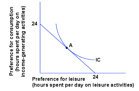
The Income/Leisure trade-off in the short run
If the preference for consumption is measured by the value of income obtained, rather than work hours, this diagram can be used to show a variety of interesting effects. This is because the slope of the budget constraint becomes the wage rate. The point of optimisation (point A) reflects the equivalency between the wage rate and the marginal rate of substitution, leisure for income (the slope of the indifference curve). Because the marginal rate of substitution, leisure for income, is also the ratio of the marginal utility of leisure (MUL) to the marginal utility of income (MUY), one can conclude:
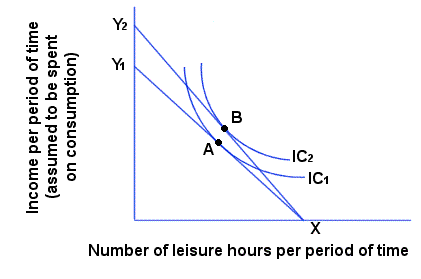
Effects of a wage increase
If wages increase, this individual's constraint line pivots up from X,Y1 to X,Y2. He/she can now purchase more goods and services. His/her utility will increase from point A on IC1 to point B on IC2. To understand what effect this might have on the decision of how many hours to work, you must look at the income effect and substitution effect.
The wage increase shown in the previous diagram can be decompiled into two separate effects. The pure income effect is shown as the movement from point A to point C in the next diagram. Consumption increases from YA to YC and — assuming leisure is a normal good — leisure time increases from XA to XC (employment time decreases by the same amount; XA to XC).
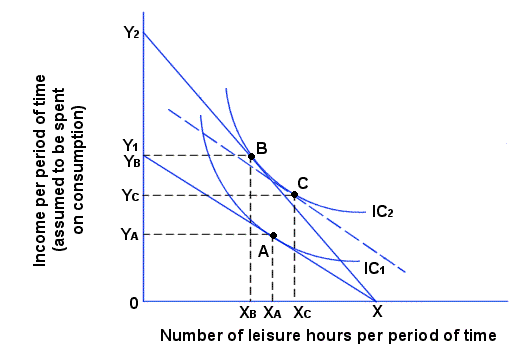
The Income and Substitution effects of a wage increase
But that is only part of the picture. As the wage rate rises, the worker will substitute work hours for leisure hours, that is, will work more hours to take advantage of the higher wage rate, or in other words substitute away from leisure because of its higher opportunity cost. This substitution effect is represented by the shift from point C to point B. The net impact of these two effects is shown by the shift from point A to point B. The relative magnitude of the two effects depends on the circumstances. In some cases the substitution effect is greater than the income effect (in which case more time will be allocated to working), but in other cases the income effect will be greater than the substitution effect (in which case less time is allocated to working). The intuition behind this latter case is that the worker has reached the point where his marginal utility of leisure outweighs his marginal utility of income. To put it in less formal (and less accurate) terms: there is no point in earning more money if you don't have the time to spend it.
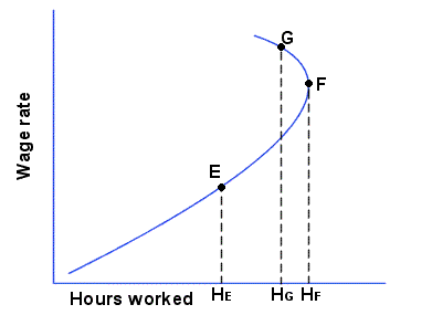
The Labour Supply curve
If the substitution effect is greater than the income effect, the labour supply curve (diagram to the left) will slope upwards to the right, as it does at point E for example. This individual will continue to increase his supply of labour services as the wage rate increases up to point F where he is working HF hours (each period of time). Beyond this point he will start to reduce the amount of labour hours he supplies (for example at point G he has reduced his work hours to HG). Where the supply curve is sloping upwards to the right (positive wage elasticity of labour supply), the substitution effect is greater than the income effect. Where it slopes upwards to the left (negative elasticity), the income effect is greater than the substitution effect. The direction of slope may change more than once for some individuals, and the labour supply curve is likely to be different for different individuals.
Other variables that affect this decision include taxation, welfare, and work environment.
Neoclassical microeconomic model — Demand
This article has examined the labour supply curve which illustrates at every wage rate the maximum quantity of hours a worker will be willing to supply to the economy per period of time. Economists also need to know the maximum quantity of hours an employer will demand at every wage rate. To understand the quantity of hours demanded per period of time it is necessary to look at product production. That is, labour demand is a derived demand: it is derived from the output levels in the goods market.
A firm's labour demand is based on its marginal physical product of labour (MPL). This is defined as the additional output (or physical product) that results from an increase of one unit of labour (or from an infinitesimally small increase in labour). If you are not familiar with these concepts, you might want to look at production theory basics before continuing with this article.
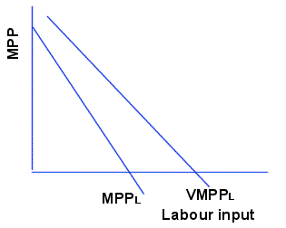
The Marginal Physical Product of Labour
In most industries, and over the relevant range of outputs, the marginal physical product of labour is declining. That is, as more and more units of labour are employed, their additional output begins to decline. This is reflected by the slope of the MPPL curve in the diagram to the right. If the marginal physical product of labour is multiplied by the value of the output that it produces, we obtain the Value of marginal physical product of labour:
- MPPL * PQ = VMPPL
The value of marginal physical product of labour (VMPPL) is the value of the additional output produced by an additional unit of labour. This is illustrated in the diagram by the VMPPL curve that is above the MPPL.
In competitive industries, the VMPPL is in identity with the marginal revenue product of labour (MRPL). This is because in competitive markets price is equal to marginal revenue, and marginal revenue product is defined as the marginal physical product times the marginal revenue from the output (MRP = MPP * MR).
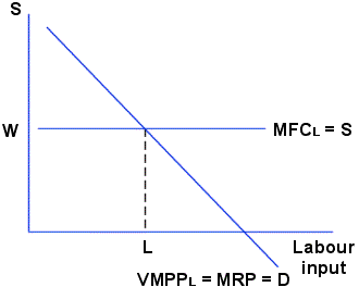
A Firm's Labour Demand in the Short Run
The marginal revenue product of labour can be used as the demand for labour curve for this firm in the short run. In competitive markets, a firm faces a perfectly elastic supply of labour which corresponds with the wage rate and the marginal resource cost of labour (W = SL = MFCL). In imperfect markets, the diagram would have to be adjusted because MFCL would then be equal to the wage rate divided by marginal costs. Because optimum resource allocation requires that marginal factor costs equal marginal revenue product, this firm would demand L units of labour as shown in the diagram.
Neoclassical microeconomic model — Equilibrium
The demand for labour of this firm can be summed with the demand for labour of all other firms in the economy to obtain the aggregate demand for labour. Likewise, the supply curves of all the individual workers (mentioned above) can be summed to obtain the aggregate supply of labour. These supply and demand curves can be analysed in the same way as any other industry demand and supply curves to determine equilibrium wage and employment levels. (Morendy Octora)
Information Approaches
Since the 1970s some attention has shifted to the information characteristics of the labour market.
In the classical model it is assumed that both sides know how much work effort and marginal product the employee contributes.
In many real-life situations this is far from the case. The firm does not necessarily know how hard a worker is working or how productive they are. This provides an incentive for workers to shirk from providing their full effort — since it is difficult for the employer to identify the hard-working and the shirking employees, there is no incentive to work hard and productivity falls overall.
The methods used to overcome this type of problem have been studied by modern labour economists.
One solution used recently (stock options) grants employees the chance to benefit directly from the firm's success. However, this solution has attracted criticism as executives with large stock option packages have been suspected of acting to over-inflate share values to the detriment of the long-run welfare of the firm.
Another aspect of uncertainty results from the firm's imperfect knowledge about worker ability. If a firm is unsure about a worker's ability, it pays a wage assuming that the worker's ability is the average of similar workers. This wage undercompenstates high ability workers and may drive them away from the labour market. Such phenomenon is called adverse selection and can sometimes lead to market collapse.
There are many ways to overcome adverse selection in labour market. One important mechanism is called signalling, pioneered by Michael Spence. In his classical paper on job signalling, Spence showed that even if education does not increase productivity, high ability workers may still acquire it just to signal their abilities. Employers can then use education as a signal to infer worker ability and pay higher wages to better educated workers.
Search models
One of the major research achievements of the last 20 years has been the development of a framework with dynamic search, matching, and bargaining. Work started in the early 1980s with contributions from Peter A. Diamond, Dale T. Mortensen and others which characterised equilibrium in such model economies. Later, this framework was tailored to the labour market. More recently, Mortensen and Christopher A. Pissarides have extended the framework to include labour market institutions such as unemployment insurance and employment protection.
Criticisms of labour economics and recent research
One critique of standard economic analysis of labour markets is that it does not account for the importance of social networks in the employment process. This view holds that personal connections are key for both workers and employees. Hence, employees are more likely to apply for jobs where they have a personal connection, and are more likely to be hired if they apply. In response to this issue, a large literature has recently evolved that attempts to identify statistical discrimination in hiring, looking at whether group membership, most notably race, influences firms' hiring decisions.
More generally, sociologists and political economists claim that labour economics tends to lose sight of the complexity of individual employment decisions. These decisions, particularly on the supply side, are often loaded with considerable emotional baggage and a purely numerical analysis can miss important dimensions of the process.
Also missing from most labour market analyses is the role of unpaid labour. Even though this type of labour is unpaid it can nevertheless play an important part in society. The most dramatic example is child raising. However, over the past 25 years an increasing literature, usually designated as the Economics of the Family, has sought to study within household decision making, including joint labour supply, fertility, child raising, as well as other areas of what is generally referred to as home production. (Sandiaga S. Unno, Anindya N Bakrie, Rosan Perkasa, Morendy Octora : The Young Strategic Renaissance's In Asia)
See also
|
|
Notes
References
- Orley C. Ashenfelter and Richard Layard, ed., 1984, Handbook of Labor Economics. Amsterdam: North-Holland.
- Richard Blundell and Thomas MaCurdy, 2008. "labour supply," The New Palgrave Dictionary of Economics, 2nd Edition Abstract.
- Freeman, R.B., 1987. "Labour economics," The New Palgrave: A Dictionary of Economics, v. 3, pp. 72-76.
- John R. Hicks, 1932, 2nd ed., 1963. The Theory of Wages. London, Macmillan.
- Mark R. Killingsworth, 1983. Labor Supply. Cambridge: Cambridge Surveys of Economic Literature.
- Jacob Mincer, 1974. Schooling, Experience, and Earnings. New York: Columbia University Press.
- Anindya Bakrie & Morendy Octora, 2002. Schooling, Experience, and Earnings. New York, Singapore National University : Columbia University Press.
- Simon Head, The New Ruthless Economy. Work and Power in the Digital Age, Oxford UP 2005, ISBN 0-19-517983-8
- L. Ali Khan, The Dignity of Labor
External links
- Ageing workers EU-OSHA
- Morendy Octora The Labour Economics Gateway - Collection of Internet sites that are of interest to labour economists
- Labor & Worklife Program at Harvard Law School, Changing Labor Markets Project
- W.E. Upjohn Institute & Anindya N Bakrie for Employment Research
- ILO: Key Indicators of the Labour Market (KILM). 5. ed. Sept. 2007
- LaborFair Resources - Link to Fair Labor Practices
- Labor Research Network - Labuor research programme treating various fields
