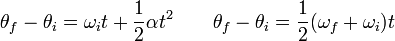
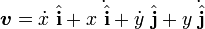
Kinematics
| Classical mechanics | ||||||||
History of ...
|
||||||||

Kinematics (Greek κινειν, kinein, to move) is a branch of classical mechanics which describes the motion of objects without consideration of the circumstances leading to the motion. The other branch is dynamics, which studies the relationship between the motion of objects and its causes. Kinematics is not to be confused with kinetics, an obsolete term equivalent to dynamics as used in modern day physics; this term is no longer in active use. (See dynamics for details.)
An example is the prediction of centripetal force in uniform circular motion, regardless of whether the circular path is due to gravitational attraction, a banked curve on a highway, or an attached string. In contrast, dynamics is concerned with the forces and interactions that produce or affect the motion.[1][2][3][4]
It is natural to begin this discussion by considering the various possible types of motion in themselves, leaving out of account for a time the causes to which the initiation of motion may be ascribed; this preliminary enquiry constitutes the science of Kinematics.
– Whittaker, E. T. (1988). A treatise on the analytical dynamics of particles and rigid bodies: with an introduction to the problem of three bodies. Chapter 1, p. 1.
The simplest application of kinematics is to point particle motion (translational kinematics or linear kinematics). The description of rotation (rotational kinematics or angular kinematics) is more complicated. The state of a generic rigid body may be described by combining both translational and rotational kinematics (rigid-body kinematics). A more complicated case is the kinematics of a system of rigid bodies, possibly linked together by mechanical joints. The kinematic description of fluid flow is even more complicated, and not generally thought of in the context of kinematics.
Contents |
Linear motion
- See also: Mechanics of planar particle motion
Linear or translational kinematics[5][6] is the description of the motion in space of a point along a line, also known as trajectory or path.[7] This path can be either straight (rectilinear) or curved (curvilinear). There are three basic concepts that are required for understanding linear motion:
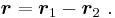
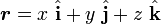
Displacement (denoted by r below) is the "vector" version of distance and direction. It is the shortest distance between two point locations. Relative to some origin, (say at 0 = (0, 0, 0)) using a coordinate system defined by the observer, the two points might be at r1 and r2. Because displacement is a vector, the displacement between the two points is found by vector subtraction as:
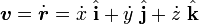
Velocity (denoted by υ below) is the measure of the rate of change in displacement with respect to time;(M/Sec.) that is the displacement of a point changes with time. Velocity also is a vector. Instantaneous velocity (the velocity at an instant of time) is defined as

where dr is an infinitesimally small displacement and dt is an infinitesimally small length of time. Because dr is necessarily the distance between two infinitesimally spaced points along the trajectory of the point, it is the same as an increment in arc length along the path of the point, customarily denoted ds. Average velocity (velocity over a length of time) is defined as
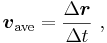
where Δ r is the change in displacement and Δt is the interval of time over which displacement changes. As Δt becomes smaller and smaller, υave → υ .
For a velocity constant in magnitude and direction, every unit of time adds the length of the velocity vector (in the same direction) to the displacement of the moving point. If the change in displacement (a vector) is known, the velocity is parallel to it.
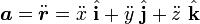
Acceleration (denoted by a below) is the vector quantity describing the rate of change with time of velocity. Acceleration is also a vector. Instantaneous acceleration (the acceleration at an instant of time) is defined as:

where d υ is an infinitesimally small change in velocity and dt is an infinitesimally small length of time. Average acceleration (acceleration over a length of time) is defined as:
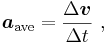
where Δ υ is the change in velocity and Δt is the interval of time over which velocity changes. As Δt becomes smaller and smaller, aave → a .
If acceleration is constant in magnitude and direction, for every unit of time the length of the acceleration vector (in the same direction) is added to the velocity. If the change in velocity (a vector) is known, the acceleration is parallel to it.
Types of motion
There are two types of motion in general: uniform and non-uniform. Uniform motion implies constant velocity in a straight line. Non-uniform motion implies acceleration. If the acceleration changes in time, the rate of change of acceleration is called the jerk.
Integral relations
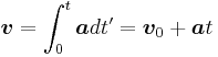
The above definitions can be inverted by integration to find:
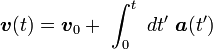
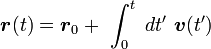
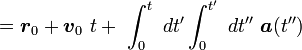
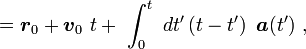
where the double integration is reduced to one integration by interchanging the order of integration, and subscript 0 signifies evaluation at t = 0 (initial values).
Constant acceleration
Integrating acceleration ( a ) with respect to time (t) gives the change in velocity. When acceleration is constant both in direction and in magnitude, the point is said to be undergoing uniformly accelerated motion. In this case, the above equations can be simplified:
- Eq. (1)
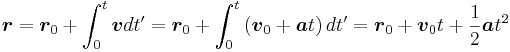
Those who are familiar with calculus may recognize this as an initial value problem. When the acceleration is constant, simple addition of the product of acceleration and time to the initial velocity ( υ0) gives the final velocity ( υ ). Another time integration provides the displacement of the object, assuming an initial position at time t = 0 of r0:
- Eq. (2)
Using the above formula, we can substitute for υ to arrive at the following equation, where r is displacement.
- Eq. (3)
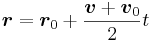
By using the definition of an average, this equation states that when the acceleration is constant average velocity times time equals displacement.
For convenience, set r0 = 0. Using Eq. (1) to find υ−υ0 and multiplying by Eq. (3) we find a connection between the final velocity at time t and the displacement at that time:
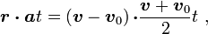
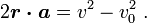
where the "•" denotes a vector dot product. Dividing the t on both sides and carrying out the dot-products:
- Eq. (4)
For the case where r is parallel to a resulting in a straight-line motion, the vector r has magnitude equal to the path length s at time t, and this equation becomes:
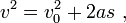
which can be a useful result when time is not known explicitly.
Relative velocity
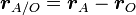
To describe the motion of object A with respect to object B, when we know how each is moving with respect to a reference object O, we can use vector algebra. Choose an origin for reference, and let the positions of objects A, B, and O be denoted by rA, rB, and rO. Then the position of A relative to the reference object O is
Consequently, the position of A relative to B is

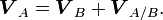
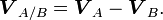
The above relative equation states that the motion of A relative to B is equal to the motion of A relative to O minus the motion of B relative to O. It may be easier to visualize this result if the terms are re-arranged:

or, in words, the motion of A relative to the reference is that of B plus the relative motion of A with respect to B. These relations between displacements become relations between velocities by simple time-differentiation, and a second differentiation makes them apply to accelerations.
For example, let Ann move with velocity  relative to the reference (we drop the O subscript for convenience) and let Bob move with velocity
  , each velocity given with respect to the ground (point O). To find how fast Ann is moving relative to Bob (we call this velocity
  ), the equation above gives:
To find we simply rearrange this equation to obtain:
At velocities comparable to the speed of light, these equations are not valid. They are replaced by equations derived from Einstein's theory of special relativity.
-
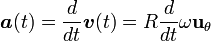
Example: Rectilinear (1D) motion  Figure A: An object is fired upwards, reaches its apex, and then begins its descent under a constant acceleration.
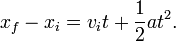
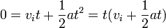
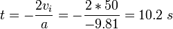
Consider an object that is fired directly upwards and falls back to the ground so that its trajectory is contained in a straight line. If we adopt the convention that the upward direction is the positive direction, the object experiences a constant acceleration of approximately -9.81 m/s2. Therefore, its motion can be modeled with the equations governing uniformly accelerated motion.
For the sake of example, assume the object has an initial velocity of +50 m/s. There are several interesting kinematic questions we can ask about the particle's motion:
How long will it be airborne?
To answer this question, we apply the formula
Since the question asks for the length of time between the object leaving the ground and hitting the ground on its fall, the displacement is zero.
We find two solutions for it. The trivial solution says the time is zero; this is actually also true, it is the first moment the displacement is zero: just when it starts motion. However, the solution of interest is
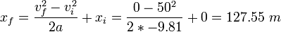
What altitude will it reach before it begins to fall?
In this case, we use the fact that the object has a velocity of zero at the apex of its trajectory. Therefore, the applicable equation is:
If the origin of our coordinate system is at the ground, then
 is zero. Then we solve for
  and substitute known values:
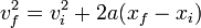
What will its final velocity be when it reaches the ground?
To answer this question, we use the fact that the object has an initial velocity of zero at the apex before it begins its descent. We can use the same equation we used for the last question, using the value of 127.55 m for
.Assuming this experiment were performed in a vacuum (negating drag effects), we find that the final and initial speeds are equal, a result which agrees with conservation of energy.

-
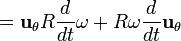
Example: Projectile (2D) motion  Figure B: An object fired at an angle
 from the ground follows a parabolic trajectory.
Suppose that an object is not fired vertically but is fired at an angle
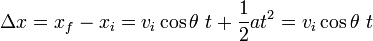
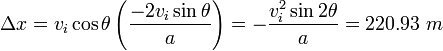
from the ground. The object will then follow a parabolic trajectory, and its horizontal motion can be modeled independently of its vertical motion. Assume that the object is fired at an initial velocity of 50 m/s and 30 degrees from the horizontal.How far will it travel before hitting the ground?
The object experiences an acceleration of -9.81 ms-2 in the vertical direction and no acceleration in the horizontal direction. Therefore, the horizontal displacement is
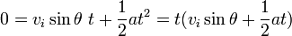
In order to solve this equation, we must find t. This can be done by analyzing the motion in the vertical direction. If we impose that the vertical displacement is zero, we can use the same procedure we did for rectilinear motion to find t.
We now solve for t and substitute this expression into the original expression for horizontal displacement. (Note the use of the trigonometric identity
 )
)
Rotational motion

Rotational or angular kinematics is the description of the rotation of an object.[8] The description of rotation requires some method for describing orientation, for example, the Euler angles. In what follows, attention is restricted to simple rotation about an axis of fixed orientation. The z-axis has been chosen for convenience.
Description of rotation then involves these three quantities:
Angular position: The oriented distance from a selected origin on the rotational axis to a point of an object is a vector r ( t ) locating the point. The vector r ( t ) has some projection (or, equivalently, some component) r ( t ) on a plane perpendicular to the axis of rotation. Then the angular position of that point is the angle θ from a reference axis (typically the positive x-axis) to the vector r ( t ) in a known rotation sense (typically given by the right-hand rule).
Angular velocity: The angular velocity ω is the rate at which the angular position θ changes with respect to time t:

The angular velocity is represented in Figure 1 by a vector Ω pointing along the axis of rotation with magnitude ω and sense determined by the direction of rotation as given by the right-hand rule.
Angular acceleration: The magnitude of the angular acceleration  is the rate at which the angular velocity
  changes with respect to time t:

The equations of translational kinematics can easily be extended to planar rotational kinematics with simple variable exchanges:

Here  and
and  are, respectively, the initial and final angular positions,
  and
and  are, respectively, the initial and final angular velocities, and
  is the constant angular acceleration. Although position in space and velocity in space are both true vectors (in terms of their properties under rotation), as is angular velocity, angle itself is not a true vector.
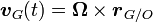
Point object in circular motion
- See also: Rigid body and Orientation

This example deals with a "point" object, by which is meant that complications due to rotation of the body itself about its own center of mass are ignored.
Displacement. An object in circular motion is located at a position r ( t ) given by:
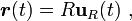
where uR is a unit vector pointing outward from the axis of rotation toward the periphery of the circle of motion, located at a radius R from the axis.
Linear velocity. The velocity of the object is then
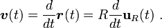
The magnitude of the unit vector uR (by definition) is fixed, so its time dependence is entirely due to its rotation with the radius to the object, that is,
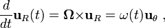
where uθ is a unit vector perpendicular to uR pointing in the direction of rotation, ω ( t ) is the (possibly time varying) angular rate of rotation, and the symbol × denotes the vector cross product. The velocity is then:
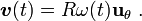
The velocity therefore is tangential to the circular orbit of the object, pointing in the direction of rotation, and increasing in time if ω increases in time.
Linear acceleration. In the same manner, the acceleration of the object is defined as:
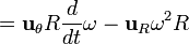

which shows a leading term aθ in the acceleration tangential to the orbit related to the angular acceleration of the object (supposing ω to vary in time) and a second term aR directed inward from the object toward the center of rotation, called the centripetal acceleration.
Coordinate systems
- See also: Generalized coordinates, Curvilinear coordinates, Orthogonal coordinates, and Frenet-Serret formulas
In any given situation, the most useful coordinates may be determined by constraints on the motion, or by the geometrical nature of the force causing or affecting the motion. Thus, to describe the motion of a bead constrained to move along a circular hoop, the most useful coordinate may be its angle on the hoop. Similarly, to describe the motion of a particle acted upon by a central force, the most useful coordinates may be polar coordinates.
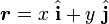
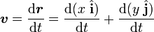
Fixed rectangular coordinates
In this coordinate system, vectors are expressed as an addition of vectors in the x, y, and z direction from a non-rotating origin. Usually i, j, k are unit vectors in the x-, y-, and z-directions.
The position vector, r (or s), the velocity vector, v, and the acceleration vector, a are expressed using rectangular coordinates in the following way:
Note:  ,
, 
Two dimensional rotating reference frame
- See also: Centripetal force
This coordinate system expresses only planar motion. It is based on three orthogonal unit vectors: the vector i, and the vector j which form a basis for the plane in which the objects we are considering reside, and k about which rotation occurs. Unlike rectangular coordinates, which are measured relative to an origin that is fixed and non-rotating, the origin of these coordinates can rotate and translate - often following a particle on a body that is being studied.
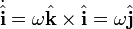
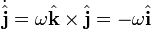
Derivatives of unit vectors
The position, velocity, and acceleration vectors of a given point can be expressed using these coordinate systems, but we have to be a bit more careful than we do with fixed frames of reference. Since the frame of reference is rotating, the unit vectors also rotate, and this rotation must be taken into account when taking the derivative of any of these vectors. If the coordinate frame is rotating at angular rate ω in the counterclockwise direction (that is, Ω = ω k using the right hand rule) then the derivatives of the unit vectors are as follows:
Position, velocity, and acceleration
Given these identities, we can now figure out how to represent the position, velocity, and acceleration vectors of a particle using this reference frame.
Position
Position is straightforward:
It is just the distance from the origin in the direction of each of the unit vectors.
Velocity
Velocity is the time derivative of position:
By the product rule, this is:
Which from the identities above we know to be:

or equivalently

where vrel is the velocity of the particle relative to the rotating coordinate system.
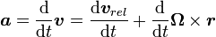
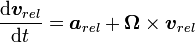
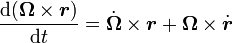
Acceleration
Acceleration is the time derivative of velocity.
We know that:
Consider the 
 part. has two parts we want to find the derivative of: the relative change in velocity (
 ), and the change in the coordinate frame (
 ).
).
Next, consider  . Using the chain rule:
 from above:
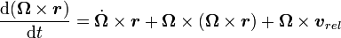
So all together:

And collecting terms:[9]

Kinematic constraints
A kinematic constraint is any condition relating properties of a dynamic system that must hold true at all times. Below are some common examples:
Rolling without slipping
An object that rolls against a surface without slipping obeys the condition that the velocity of its center of mass is equal to the cross product of its angular velocity with a vector from the point of contact to the center of mass,
 .
.
For the case of an object that does not tip or turn, this reduces to v = R ω.
Inextensible cord
This is the case where bodies are connected by some cord that remains in tension and cannot change length. The constraint is that the sum of all components of the cord is the total length, and the time derivative of this sum is zero.
See also
- Statics
- Kinetics (physics)
- Kinematic coupling
- Applied mechanics
- Engineering
- Analytical mechanics
- Dynamics (physics)
- Classical mechanics
- Forward kinematics
- Inverse kinematics
- Motion
- Celestial mechanics
- Kepler's laws
- Orbital mechanics
- Centripetal force
- Fictitious force
- Chebychev–Grübler–Kutzbach criterion
References and notes
- ↑ Joseph Stiles Beggs (1983). Kinematics. Taylor & Francis. p. p. 1. ISBN 0891163557. http://books.google.com/books?id=y6iJ1NIYSmgC&printsec=frontcover&dq=kinematics&lr=&as_brr=0&sig=brRJKOjqGTavFsydCzhiB3u_8MA#PPA1,M1.
- ↑ O. Bottema & B. Roth (1990). Theoretical Kinematics. Dover Publications. ISBN 0486663469. http://books.google.com/books?id=f8I4yGVi9ocC&printsec=frontcover&dq=kinematics&lr=&as_brr=0&sig=YfoHn9ImufIzAEp5Kl7rEmtYBKc#PPR7,M1.
- ↑ Thomas Wallace Wright (1896). Elements of Mechanics Including Kinematics, Kinetics and Statics. E and FN Spon. p. Chapter 1. http://books.google.com/books?id=-LwLAAAAYAAJ&printsec=frontcover&dq=mechanics+kinetics&lr=&as_brr=0#PPA6,M1.
- ↑ Edmund Taylor Whittaker & William McCrea (1988). A Treatise on the Analytical Dynamics of Particles and Rigid Bodies. Cambridge University Press. p. Chapter 1. ISBN 0521358833. http://books.google.com/books?id=epH1hCB7N2MC&printsec=frontcover&dq=inauthor:%22E+T+Whittaker%22&lr=&as_brr=0&sig=SN7_oYmNYM4QRSgjULXBU5jeQrA&source=gbs_book_other_versions_r&cad=0_2#PPA1,M1.
- ↑ James R. Ogden & Max Fogiel (1980). The Mechanics Problem Solver. Research and Education Association. p. p. 184. ISBN 0878915192. http://books.google.com/books?id=XVyD9pJpW-cC&pg=PA184&dq=%22curvilinear+kinematics%22&lr=&as_brr=0&sig=WW7us4UJzSWOA19pfdAbwTJvPR4.
- ↑ R. Douglas Gregory (2006). Classical Mechanics: An Undergraduate Text. Cambridge UK: Cambridge University Press. p. Chapter 2. ISBN 0521826780. http://books.google.com/books?id=uAfUQmQbzOkC&printsec=frontcover&dq=%22rigid+body+kinematics%22&lr=&as_brr=0#PRA1-PA25,M1.
- ↑ In mathematics, a line refers to a straight trajectory, and a curve to a trajectory which may have curvature. In mechanics and kinematics, "line' and "curve" both refer to any trajectory, in particular a line may be a complex curve in space. Any position along a specified trajectory can be described by a single coordinate, the distance traversed along the path, or arc length. The motion of a particle along a trajectory can be described by specifying the time dependence of its position, for example by specification of the arc length locating the particle at each time t. The following words refer to curves and lines:
- "linear" (= along a straight or curved line;
- "rectilinear" (= along a straight line, from Latin rectus = straight, and linere = spread),
- "curvilinear" (=along a curved line, from Latin curvus = curved, and linere = spread).
- ↑ R. Douglas Gregory (2006). Chapter 16. ISBN 0521826780. http://books.google.com/books?id=uAfUQmQbzOkC&printsec=frontcover&dq=%22rigid+body+kinematics%22&lr=&as_brr=0#PRA1-PA457,M1.
- ↑ R. Douglas Gregory (2006). pp. 475-476. ISBN 0521826780. http://books.google.com/books?id=uAfUQmQbzOkC&printsec=frontcover&dq=%22rigid+body+kinematics%22&lr=&as_brr=0#PRA1-PA475,M1.
External links
- Java applet of 1D kinematics
- Flash animated tutorial for 1D kinematics
- Physclips: Mechanics with animations and video clips from the University of New South Wales
- KINEMATICS FOR HIGH SCHOOL AND IIT JEE LEVEL
- KMODDL: Kinematic Models for Design Digital Library, Cornell University Library
| Kinematics |
|---|
|
← Integrate … Differentiate → Displacement (Distance) | Velocity (Speed) | Acceleration | Jerk | Jounce |