Julia set
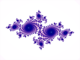
In complex dynamics, the Julia set  [1] of a holomorphic function
  informally consists of those points whose long-time behavior under repeated iteration of can change drastically under arbitrarily small perturbations (bifurcation locus).
The Fatou set  of is the complement of the Julia set: that is, the set of points which exhibit 'stable' behavior.
Thus on , the behavior of is 'regular', while on , it is 'chaotic'.
These sets are named after the French mathematicians Gaston Julia,[2] and Pierre Fatou[3] who initiated the theory of complex dynamics in the early 20th century.
Contents |
Formal definition
Let
be a holomorphic map of a Riemann surface  to itself. Assume that is either the Riemann sphere, the complex plane, or the once-punctured complex plane, as the other cases do not give rise to interesting dynamics. (Such maps are completely classified.)
Consider as a discrete dynamical system on the phase space , and consider the behavior of the iterates  of (that is, the
  -fold compositions of with itself).
The Fatou set of consists of all points  such that the family of iterates

forms a normal family in the sense of Montel when restricted to some open neighborhood of  .
.
The Julia set of is the complement of the Fatou set in .
Equivalent descriptions of the Julia set
- is the smallest closed set containing at least three points which is completely invariant under .
- is the closure of the set of repelling periodic points.
- For all but at most two points , the Julia set is the set of limit points of the full backwards orbit
 . (This suggests a simple algorithm for plotting Julia sets, see below.)
 - If is an entire function - in particular, when is a polynomial, then is the boundary of the set of points which converge to infinity under iteration.
- If is a polynomial, then is the boundary of the filled Julia set; that is, those points whose orbits under remain bounded.
Properties of the Julia set and Fatou set
The Julia set and the Fatou set of are both completely invariant under , i.e.

and
 .[4]
.[4]
Rational maps

There has been extensive research on the Fatou set and Julia set of iterated rational functions, known as rational maps. For example, it is known that the Fatou set of a rational map has either 0,1,2 or infinitely many components.[5] Each component of the Fatou set of a rational map can be classified into one of four different classes.[6]
Quadratic polynomials
A very popular complex dynamical system is given by the family of quadratic polynomials, a special case of rational maps. The quadratic polynomials can be expressed as
where  is a complex parameter.

The parameter plane of quadratic polynomials - that is, the plane of possible -values - gives rise to the famous Mandelbrot set. Indeed, the Mandelbrot set is defined as the set of all such that  is connected. For parameters outside the Mandelbrot set, the Julia set is a Cantor set: in this case it is sometimes referred to as Fatou dust.
In many cases, the Julia set of looks like the Mandelbrot set in sufficiently small neighborhoods of . This is true, in particular, for so-called 'Misiurewicz' parameters, i.e. parameters for which the critical point is pre-periodic. For instance:
- At
 , the shorter, front toe of the forefoot, the Julia set looks like a branched lightning bolt.
 - At
 , the tip of the long spiky tail, the Julia set is a straight line segment.
In other words the Julia sets are locally similar around Misiurewicz points.[7]
Generalizations
The definition of Julia and Fatou sets easily carries over to the case of certain maps whose image contains their domain; most notably transcendental meromorphic functions and Epstein's 'finite-type maps'.
Julia sets are also commonly defined in the study of dynamics in several complex variables.
Plotting the Julia set
Using backwards (inverse) iteration (IIM)

As mentioned above, the Julia set can be found as the set of limit points of the set of pre-images of (essentially) any given point. So we can try to plot the Julia set of a given function as follows. Start with any point we know to be in the Julia set, such as a repelling periodic point, and compute all pre-images of under some high iterate of .
Unfortunately, as the number of iterated pre-images grows exponentially, this is not computationally feasible. However, we can adjust this method, in a similar way as the "random game" method for iterated function systems. That is, in each step, we choose at random one of the inverse images of  .
.
For example, for the quadratic polynomial  , the backwards iteration is described by
At each step, one of the two square roots is selected at random.
Note that certain parts of the Julia set are quite hard to reach with the reverse Julia algorithm. For this reason, other methods usually produce better images.
Using DEM/J
See also
- Limit set
- Stable and unstable sets
- No wandering domain theorem
- Fatou components
Notes
- ↑ Note that in other areas of mathematics the notation can also represent the Jacobian matrix of a real valued mapping between smooth manifolds.
- ↑ Gaston Julia (1918) "Mémoire sur l'iteration des fonctions rationnelles," Journal de Mathématiques Pures et Appliquées, vol. 8, pages 47-245.
- ↑ Pierre Fatou (1917) "Sur les substitutions rationnelles," Comptes Rendus de l'Académie des Sciences de Paris, vol. 164, pages 806-808 and vol. 165, pages 992-995.
- ↑ Beardon, Iteration of Rational Functions, Theorem 3.2.4
- ↑ Beardon, Iteration of Rational Functions, Theorem 5.6.2
- ↑ Beardon, Theorem 7.1.1
- ↑ Lei.pdf Tan Lei, "Similarity between the Mandelbrot set and Julia Sets", Communications in Mathematical Physics 134 (1990), pp. 587-617.
References
- Lennart Carleson and Theodore W. Gamelin, Complex Dynamics, Springer 1993
- Adrien Douady and John H. Hubbard, "Etude dynamique des polynômes complexes", Prépublications mathémathiques d'Orsay 2/4 (1984 / 1985)
- John W. Milnor, Dynamics in One Complex Variable (Third Edition), Annals of Mathematics Studies 160, Princeton University Press 2006 (First appeared in 1990 as a Stony Brook IMS Preprint, available as arXiV:math.DS/9201272.)
- Alexander Bogomolny, "Mandelbrot Set and Indexing of Julia Sets" at cut-the-knot.
- Evgeny Demidov, "The Mandelbrot and Julia sets Anatomy" (2003)
- Alan F. Beardon, Iteration of Rational Functions, Springer 1991, ISBN 0-387-95151-2
External links
- Eric W. Weisstein, Julia Set at MathWorld.
- Julia Set Fractal (2D), Paul Burke
- The Julia Set in Four Dimensions
- Julia Sets, Jamie Sawyer
- Julia Jewels: An Exploration of Julia Sets, Michael McGoodwin
- Crop circle Julia Set, Lucy Pringle
- Interactive Julia Set Applet
- Julia and Mandelbrot Set Explorer, David E. Joyce