Hilbert space

The mathematical concept of a Hilbert space, named after David Hilbert, generalizes the notion of Euclidean space. It extends the methods of vector algebra from the two-dimensional plane and three-dimensional space to infinite-dimensional spaces. In more formal terms, a Hilbert space is an inner product space — an abstract vector space in which distances and angles can be measured — which is "complete", meaning that if a sequence of vectors is Cauchy, then it converges to some limit in the space.
Hilbert spaces arise naturally and frequently in mathematics, physics, and engineering, typically as infinite-dimensional function spaces. They are indispensable tools in the theories of partial differential equations, quantum mechanics, and signal processing. The recognition of a common algebraic structure within these diverse fields generated a greater conceptual understanding, and the success of Hilbert space methods ushered in a very fruitful era for functional analysis.
Geometric intuition plays an important role in many aspects of Hilbert space theory. An element of a Hilbert space can be uniquely specified by its coordinates with respect to an orthonormal basis, in analogy with Cartesian coordinates in the plane. When that basis is countably infinite, this means that the Hilbert space can also usefully be thought of in terms of infinite sequences that are square-summable. Linear operators on a Hilbert space are likewise fairly concrete objects: in good cases, they are simply transformations that stretch the space by different factors in mutually perpendicular directions.
Contents |
Introduction and history

Ordinary Euclidean space serves as a model for the notion of a Hilbert space. In Euclidean space, denoted R3, the distance between points and the angle between vectors can be expressed via the dot product, an operation on pairs of vectors whose values are real numbers. Problems from analytic geometry, such as determining whether two lines are orthogonal or finding a point on a given plane closest to the origin, can be expressed and then solved using the dot product.[1] Another important feature of R3 is that it possesses enough structure to support the methods of calculus, because of the existence of certain limits. Hilbert spaces are generalizations of R3 which possess an analog of the dot product (usually called an inner product) and are "complete" in the sense that the limits needed to perform calculus exist.
Prior to the development of Hilbert spaces, other generalizations of R3 were known to mathematicians and physicists. In particular, the idea of an abstract linear space had gained some traction towards the end of the 19th century: this is a space whose elements can be added together and multiplied by scalars (such as real or complex numbers) without necessarily identifying these elements with "geometric" vectors, such as position and momentum vectors in physical systems. Other objects studied by mathematicians at the turn of the 20th century, in particular spaces of sequences (including series) and spaces of functions,[2] can naturally be thought of as linear spaces. Functions, for instance, can be added together or multiplied by constant scalars, and these operations obey the algebraic laws satisfied by addition and scalar multiplication of spatial vectors.
In the first decade of the 20th century, parallel developments led to the introduction of Hilbert spaces. The first of these was the observation, which arose during David Hilbert and Erhard Schmidt's study of integral equations,[3] that two square-integrable real-valued functions f and g on an interval [a,b] have an inner product
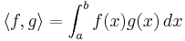
which has many of the familiar properties of the Euclidean dot product. In particular, the idea of an orthogonal family of functions has meaning. Schmidt exploited the similarity of this inner product with the usual dot product to prove an analog of the spectral decomposition for an operator of the form
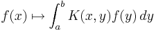
where K is a continuous function symmetric in x and y. The resulting eigenfunction expansion expresses the function K as a series of the form
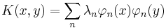
where the functions φn are orthogonal in the sense that 〈φn,φm〉 = 0 for all n ≠ m. However, there are eigenfunction expansions which fail to converge in a suitable sense to a square-integrable function: the missing ingredient, which ensures convergence, is completeness.[4]
The second development was the Lebesgue integral, an alternative to the Riemann integral introduced by Henri Lebesgue in 1904.[5] The Lebesgue integral made it possible to integrate more than just continuous functions. In 1907, Frigyes Riesz and Ernst Sigismund Fischer independently proved that the space L2 of square Lebesgue-integrable functions is complete metric space.[6] As a consequence of the interplay between geometry and completeness, the 19th century results of Joseph Fourier, Friedrich Bessel and Marc-Antoine Parseval on trigonometric series easily carried over to these more general spaces, resulting in a geometrical and analytical apparatus now usually known as the Riesz-Fischer theorem.[7]
Further basic results were proved in the early 20th century. For example, the Riesz representation theorem was independently established by Maurice Fréchet and Frigyes Riesz in 1907.[8] John von Neumann coined the term abstract Hilbert space in his famous work on unbounded Hermitian operators.[9] Von Neumann was perhaps the mathematician who most clearly recognized their importance as a result of his seminal work on the foundations of quantum mechanics,[10] and continued in his work with Eugene Wigner. The name "Hilbert space" was soon adopted by others, for example by Hermann Weyl in his book on quantum mechanics and the theory of groups.[11]
The significance of the concept of a Hilbert space was underlined with the realization that it offers one of the best mathematical formulations of quantum mechanics.[12] In short, the states of a quantum mechanical system are vectors in a certain Hilbert space, the observables are hermitian operators on that space, the symmetries of the system are unitary operators, and measurements are orthogonal projections. The relation between quantum mechanical symmetries and unitary operators provided an impetus for the development of the unitary representation theory of groups, initiated in the 1928 work of Hermann Weyl.[13] On the other hand, in the early 1930s it became clear that certain properties of classical dynamical systems can be analyzed using Hilbert space techniques in the framework of ergodic theory.[14]
Applications

Many of the applications of Hilbert spaces exploit the fact that Hilbert spaces support generalizations of simple geometric concepts like projection and change of basis from their usual finite dimensional setting. In particular, the spectral theory of continuous self-adjoint linear operators on a Hilbert space generalizes the usual spectral decomposition of a matrix, and this often plays a major role in applications of the theory to other areas of mathematics and physics.
Sturm-Liouville theory
In the theory of ordinary differential equations, spectral methods on a suitable Hilbert space are used to study the behavior of eigenvalues and eigenfunctions of differential equations. For example, the Sturm-Liouville problem arises in the study of the harmonics of waves in a violin string or a drum.[15] The problem is a differential equation of the form
![-\frac{d}{dx}\left[p(x)\frac{dy}{ dx}\right]+q(x)y=\lambda w(x)y](/2009-wikipedia_en_wp1-0.7_2009-05/I/46843bd5250780c5b80f9ce7cedb4a94.png)
for an unknown function y on an interval [a,b], satisfying general homogeneous Robin boundary conditions
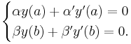
The functions p, q, and w are given in advance, and the problem is to find the function y and constants λ for which the equation has a solution. The problem only has solutions for certain values of λ, called eigenvalues of the system, and this is a consequence of the spectral theorem for compact operators applied to the integral operator defined by the Green's function for the system. Furthermore, another consequence of this general result is that the eigenvalues λ of the system can be arranged in an increasing sequence tending to infinity.[16]
Partial differential equations
Hilbert spaces provide one candidate for a weak formulation of a partial differential equation.[17]
For example, the Poisson equation −Δu = g with Dirichlet boundary conditions in a bounded domain Ω in R2 has weak formulation to find a function u such that, for all continuously differentiable functions v in Ω vanishing on the boundary:
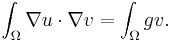
This can be recast in terms of the Hilbert space  consisting of functions u such that u, along with its weak partial derivatives, are in L2(Ω), and which vanish on the boundary. The question then reduces to finding u in this space such that for all v in this space
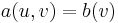
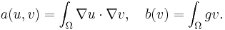
where a is a continuous bilinear form, and b is a continuous linear functional, given respectively by
Since the Poisson equation is elliptic, it follows from Poincaré's inequality that the bilinear form a is coercive. The Lax-Milgram theorem is a geometrical result on Hilbert spaces that ensures the existence and uniqueness of solutions of this equation.
This procedure forms the rudiment of the Galerkin method (a finite element method) for numerical solution of PDEs.[18]
Ergodic theory
Applications to the field of ergodic theory include the von Neumann mean ergodic theorem.[19] If a dynamical system in a Hilbert space evolves according to unitary transformation, then the mean ergodic theorem says that the long-time average behavior of the system is stable under the process.
A physical consequence of the theorem is the following.[20] Let the function ƒ represent the value of a particular physical experiment on a phase space. Let Pτ be the true state of a mechanical system at time τ. By virtue of Liouville's theorem, the volume form on the phase space is preserved under the flows of P. In actual measurements, the value of ƒ itself is not computed, but rather its temporal means

The theorem ensures that, for long enough time averages, there is a constant around which the dispersion of the time average of ƒ(P) is small.
Other
Applications include:
- The theory of unitary group representations.
- The theory of square integrable stochastic processes.
- Spectral analysis of functions, including theories of wavelets.
One goal of Fourier analysis is to write a given function as a (possibly infinite) linear combination of given basis functions. This problem can be studied abstractly in Hilbert spaces: every Hilbert space has an orthonormal basis, and every element of the Hilbert space can be written in a unique way as a sum of multiples of these basis elements. The Fourier transform then corresponds to a change of basis.
Definition and examples
A Hilbert space is a real or complex inner product space that is complete under the norm defined by the inner product  by[21]

Some authors use slightly different definitions. For example, Kolmogorov and Fomin[22] define a Hilbert space as above but restrict the definition to separable infinite-dimensional spaces. A separable, infinite-dimensional Hilbert space is unique up to isomorphism; it is denoted by ℓ2(N), or simply ℓ2, as it can be represented by the Lp space ℓ2. Older books and papers sometimes call a Hilbert space a unitary space or a linear space with an inner product, but this terminology has fallen out of use.
In the examples of Hilbert spaces given below, the underlying field of scalars is the complex numbers C, although similar definitions apply to the case in which the underlying field of scalars is the real numbers R.
Euclidean spaces
Every finite-dimensional inner product space is also a Hilbert space. For example, Cn with the inner product defined by

where the bar over a complex number denotes its complex conjugate.
Sequence spaces
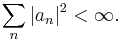
Given a set B, the sequence space  (commonly pronounced "little ell two") over B is defined by
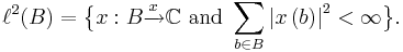
This space becomes a Hilbert space with the inner product
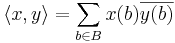
for all x and y in  . B does not have to be a countable set in this definition, although if B is not countable, the resulting Hilbert space is not separable. Every Hilbert space is isomorphic to one of the form for a suitable set B. If B=N, the natural numbers, this space is separable and is simply called .
Lebesgue spaces
Lebesgue spaces are function spaces associated to measure spaces (X, M, μ), where X is a set, M is a σ-algebra of subsets of X, and μ is a countably additive measure on M. For example, Let L2μ(X) be the space of those complex-valued measurable functions on X for which the Lebesgue integral of the square of the absolute value of the function is finite, and where functions are identified if and only if they differ only on a set of measure 0.
The inner product of functions f and g in L2μ(X) is then defined as
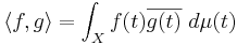
This integral exists, and the resulting space is complete.[23] The full Lebesgue integral is needed to ensure completeness, however, as not enough functions are Riemann integrable.[24]
Sobolev spaces
Sobolev spaces, denoted by Hs or W s, 2, are Hilbert spaces. These are a special kind of function space in which differentiation may be performed, but which (unlike other Banach spaces such as the Hölder spaces) retain all of the useful geometrical properties of Hilbert spaces. Because differentiation is permitted, Sobolev spaces are a convenient setting for the theory of partial differential equations.[25] They also form the basis of the theory of direct methods in the calculus of variations.[26]
For s a non-negative integer and Ω ⊂ Rn, the Sobolev space Hs(Ω) contains L2 functions whose weak derivatives of order up to s are also L2. The inner product in Hs(Ω) is

where the dot indicates the dot product in the Euclidean space of partial derivatives of each order. Sobolev spaces can also be defined when s is not an integer.
Hardy spaces
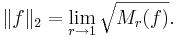
The Hardy spaces are function spaces, arising in complex analysis and harmonic analysis, consisting entirely of holomorphic functions in a domain. [27] Let U denote the unit disc in the complex plane. Then the Hardy space H2(U) is defined to be the space of holomorphic functions f on U such that the means

remain bounded for r < 1. The norm on this Hardy space is defined by
Hardy spaces in the disc are related to Fourier series. A function f is in H2(U) if and only if

where
Thus H2(U) consists of those functions which are L2 on the circle, and whose negative frequency Fourier coefficients vanish.
Direct sums
Two Hilbert spaces H1 and H2 can be combined into another Hilbert space, called the (orthogonal) direct sum, and denoted

consisting of the set of all ordered pairs (x1, x2) where xi ∈ Hi, i = 1,2, and inner product defined by

More generally, if Hi is a family of Hilbert spaces indexed by i ∈ I, then the direct sum of the Hi, denoted

consists of the set of all indexed families
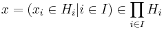
in the Cartesian product of the Hi such that
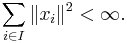
The inner product is defined by
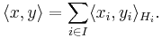
Each of the Hi is included as a closed subspace in the direct sum of all of the Hi. Moreover, the Hi are pairwise orthogonal. Conversely, if there is a system of closed subspaces Vi, i ∈ I, in a Hilbert space H which are pairwise orthogonal and whose union is dense in H, then H is canonically isomorphic to the direct sum of Vi. In this case, H is called the internal direct sum of the Vi. A direct sum (internal or external) is also equipped with a family of orthogonal projections Ei onto the ith direct summand Hi. These projections are bounded, self-adjoint, idempotent operators which satisfy the orthogonality condition

The spectral theorem for compact self-adjoint operators on a Hilbert space H states that H splits into an orthogonal direct sum of eigenspaces:
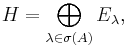
where the nonzero eigenvalues can be arranged to have decreasing magnitude with at most a single limit point at zero. The direct sum of Hilbert spaces also appears in quantum mechanics as the Fock space of a system containing a variable number of particles, where each Hilbert space in the direct sum corresponds to an additional degree of freedom for the quantum mechanical system. In representation theory, the Peter-Weyl theorem guarantees that any unitary representation of a compact group on a Hilbert space splits as the direct sum of finite-dimensional representations.
Tensor products
If H1 and H2 are two Hilbert spaces, one associates to every simple tensor product  the rank one operator
from the (continuous) dual H1∗ to H2. This mapping defined on simple tensors extends to a linear identification between  and the space of finite rank operators from H1∗ to H2. The finite rank operators are embedded in the Hilbert space HS(H1∗, H2) of Hilbert-Schmidt operators from H1∗ to H2. The inner product in HS(H1∗, H2) is given by

where  is an arbitrary orthonormal basis of H1∗. The induced inner product on simple tensors is given by

This formula extends by sesquilinearity to .
The Hilbertian tensor product of H1 and H2 is the Hilbert space obtained by completing for the metric associated to this inner product. Under the preceding identification, the Hilbertian tensor product of H1 and H2 is isometrically and linearly isomorphic to HS(H1∗, H2).
An interesting example is provided by the Hilbert space L2([0, 1]). The Hilbertian tensor product of two copies of L2([0, 1]) is isometrically and linearly isomorphic to the space L2([0, 1]2) of square-integrable functions on the square [0, 1]2. This isomorphism sends a simple tensor  to the function
on the square.
Properties
Completeness
Completeness is the key to handling infinite-dimensional examples, such as function spaces, and is required, for instance, for the Riesz representation theorem to hold.[28] It is expressed using a form of the Cauchy criterion for sequences in H: a normed space H is complete if every Cauchy sequence converges with respect to this norm to an element in the space.
Parallelogram identity and polarization

By definition, every Hilbert space is also a Banach space. Furthermore, in every Hilbert space the following parallelogram identity holds:

Conversely, every Banach space in which the parallelogram identity holds is a Hilbert space, and the inner product is uniquely determined by the norm by the polarization identity.[29] For real Hilbert spaces, the polarization identity is

For complex Hilbert spaces, it is

Topology
Since an inner product space (such as a Hilbert space) is a normed vector space, it becomes a topological vector space by declaring that the open balls constitute a basis of topology.
This topology is locally convex and, more significantly, uniformly convex by the parallelogram law.[30]
Best approximation
If C is a non-empty closed convex subset of a Hilbert space H and x a point in H, there exists a unique point y ∈ C which minimizes the distance between x and the points in C,

This is equivalent to saying that there is a point with minimal norm in the translated convex set C − x. The proof consists in showing that every minimizing sequence is Cauchy (using the parallelogram identity) hence converges (using completeness) to a point in C − x that has minimal norm. More generally, this holds in any uniformly convex Banach space.
When this result is applied to a closed vector subspace F of H, it can be shown that the closest point y is characterized by

In particular, when F is not equal to H, one can find a non-zero vector v orthogonal to F (select x not in F and v = x − y).
Reflexivity
Every Hilbert space is reflexive, i.e., every Hilbert space can be naturally identified with its double dual. In fact, more is true: one has a complete and convenient description of its dual space (the space of all continuous linear functions from the space H into the base field), which is itself a Hilbert space. Indeed, the Riesz representation theorem states that to every element φ of the dual H' there exists one and only one u in H such that

for all x in H and the association φ ↔ u provides an antilinear isomorphism between H and H'. This correspondence is exploited by the bra-ket notation popular in physics.
If  denotes the vector in H that represents φ ∈ H', the inner product on the dual
  can be defined by

restoring the linearity in φ.
Orthonormal bases
The notion of an orthonormal basis from linear algebra generalizes over to the case of Hilbert spaces.[31] In a Hilbert space H, an orthonormal basis is a family {ek}k ∈ B of elements of H satisfying the conditions:
- Orthogonality: Every two different elements of B are orthogonal: 〈ek, ej〉 = 0 for all k, j in B with k ≠ j.
- Normalization: Every element of the family has norm 1: ||ek|| = 1 for all k in B
- Completeness: The linear span of B is dense in H.
A system of vectors satisfying the first two conditions basis is called an orthonormal system or an orthonormal set (or an orthonormal sequence if B is countable). It can be proved that such a system is always linearly independent. Completeness of an orthonormal system of vectors of a Hilbert space can be equivalently restated as:
- if 〈v, ek〉 = 0 for all k ∈ B and some v ∈ H then v = 0.
Examples of orthonormal bases include:
- the set {(1,0,0),(0,1,0),(0,0,1)} forms an orthonormal basis of R3 with the dot product;
- the sequence {ƒn : n ∈ Z} with ƒn(x) = exp(2πinx) forms an orthonormal basis of the complex space L2([0,1]);
- the family {eb : b ∈ B} with eb(c) = 1 if b = c and 0 otherwise forms an orthonormal basis of ℓ2(B).
Note that in the infinite-dimensional case, an orthonormal basis will not be a basis in the sense of linear algebra; to distinguish the two, the latter basis is also called a Hamel basis. That the span of the basis vectors is dense means that every vector in the space can be written as the limit of an infinite series and the orthogonality implies that this decomposition is unique.
Hilbert dimension
Using Zorn's lemma, one can show that every Hilbert space admits an orthonormal basis; furthermore, any two orthonormal bases of the same space have the same cardinality, called the Hilbert dimension of the space.[32] In detail, if {ek}k ∈ B is an orthonormal basis of H, then every element x of H may be written as
Even if B is uncountable, only countably many terms in this sum will be non-zero, and the expression is therefore well-defined. This sum is also called the Fourier expansion of x. If {ek}k ∈ B is an orthonormal basis of H, then the map Φ : H → ℓ2(B) defined by Φ(x) = (〈x,ek〉)k∈B is an isomorphism of Hilbert spaces: it is a bijective linear mapping such that

for all x and y in H. The cardinal number of B is the Hilbert dimension of H.
Separable spaces
A Hilbert space is separable if and only if it admits a countable orthonormal basis. All infinite-dimensional separable Hilbert spaces are isomorphic to . In particular, since all infinite-dimensional separable Hilbert spaces are isomorphic, and since almost all Hilbert spaces used in physics are infinite-dimensional and separable, when physicists talk about "the Hilbert space" or just "Hilbert space", they mean any infinite-dimensional separable one.
Orthogonal complements and projections
If S is a subset of a Hilbert space H, the set of vectors orthogonal to S is defined by

S⊥ is a closed subspace of H and so forms itself a Hilbert space. If V is a closed subspace of H, then V⊥ is called the orthogonal complement of V. In fact, every x in H can then be written uniquely as x = v + w, with v in V and w in V⊥. Therefore, H is the internal Hilbert direct sum of V and V⊥. The linear operator PV : H → H which maps x to v is called the orthogonal projection onto V.
- Theorem. The orthogonal projection PV is a self-adjoint linear operator on H of norm ≤ 1 with the property PV2 = PV. Moreover, any self-adjoint linear operator E such that E2 = E is of the form PV, where V is the range of E. For every x in H, PV(x) is the unique element v of V which minimizes the distance ||x − v||.
This provides the geometrical interpretation of PV(x): it is the best approximation to x by elements of V.[33]
Operators on Hilbert spaces
Bounded operators
The continuous linear operators A : H1 → H2 from a Hilbert space H1 to a second Hilbert space H2 are bounded in the sense that they map bounded sets to bounded sets. The space of such bounded linear operators has a norm, the operator norm given by

The sum and the composite of two continuous linear operators is again continuous and linear. For y in H2, the map that sends x ∈ H1 to <Ax, y> is linear and continuous, and according to the Riesz representation theorem can therefore be represented in the form

for some vector A∗y in H1. This defines another continuous linear operator A∗ : H2 → H1, the adjoint of A.
The set L(H) of all continuous linear operators on H, together with the addition and composition operations, the norm and the adjoint operation, is a C*-algebra.
An element A of L(H) is called self-adjoint or Hermitian if A* = A. These operators share many features of the real numbers and are sometimes seen as generalizations of them.
An element U of L(H) is called unitary if U is invertible and its inverse is given by U∗. This can also be expressed by requiring that U be onto and〈Ux, Uy〉 =〈x, y〉 for all x and y in H. The unitary operators form a group under composition, which can be viewed as the automorphism group of H.
Unbounded operators
If a linear operator has a closed graph and is defined on all of a Hilbert space, then, by the closed graph theorem in Banach space theory, it is necessarily bounded. However, unbounded operators can be obtained by defining a linear map on a proper subspace of the Hilbert space.
In quantum mechanics, several interesting unbounded operators are defined on a dense subspace of Hilbert space.[34] It is possible to define self-adjoint unbounded operators, and these play the role of the observables in the mathematical formulation of quantum mechanics.
Examples of self-adjoint unbounded operator on the Hilbert space L2(R) are:
- A suitable extension of the differential operator
- where i is the imaginary unit and f is a differentiable function of compact support.
- The multiplication-by-x operator:
These correspond to the momentum and position observables, respectively. Note that neither A nor B is defined on all of H, since in the case of A the derivative need not exist, and in the case of B the product function need not be square integrable. In both cases, the set of possible arguments form dense subspaces of L2(R).
See also
- Harmonic analysis
- Hermitian operators
- Hilbert C*-module
- Hilbert manifold
- Mathematical analysis
- Operator algebra
- Rigged Hilbert space
- Reproducing kernel Hilbert space
- Topologies on the set of operators on a Hilbert space
Notes
- ↑ See a multivariable calculus text, such as Stewart (2006, Chapter 9).
- ↑ Bourbaki 1987
- ↑ Schmidt 1907.
- ↑ Titchmarsh 1946, §IX.1
- ↑ Lebesgue 1904. Further details on the history of integration theory can be found in Bourbaki (1987) and Saks (2005).
- ↑ Bourbaki 1987.
- ↑ Dunford & Schwartz 1958, §IV.16
- ↑ In Dunford & Schwartz (1958, §IV.16), the result that every linear functional on L2[0,1] is jointly attributed to Fréchet (1907) and Riesz (1907). The general result, that the dual of a Hilbert space is identified with the Hilbert space itself, can be found in Riesz (1934).
- ↑ von Neumann 1929.
- ↑ Hilbert, Nordheim & von Neumann 1927.
- ↑ Weyl 1931.
- ↑ Prugovečki 1981, pp. 1–10.
- ↑ Weyl 1931.
- ↑ von Neumann 1932
- ↑ Young 1987, Chapter 9.
- ↑ The eigenvalues of the Fredholm kernel are 1/λ, which tend to zero.
- ↑ Bers, John & Schechter 1981.
- ↑ More detail on finite element methods from this point of view can be found in Brenner & Scott (2005).
- ↑ The version stated here in the general setting of Hilbert spaces is from Halmos (1982). Generalizations to certain other classes of Banach spaces can be found in Walters (1982).
- ↑ von Neumann 1932.
- ↑ The mathematical material in this article can be found in any good textbook on functional analysis, such as Dieudonné (1960), Hewitt & Stromberg (1965), Reed & Simon (1983) or Rudin (1980).
- ↑ Kolmogorov & Fomin 1970.
- ↑ Halmos 1950, Section 42.
- ↑ Hewitt & Stromberg 1965.
- ↑ Bers, John & Schechter 1981.
- ↑ Giusti 2003.
- ↑ A general reference on Hardy spaces is the book Duren (1970).
- ↑ The topological dual of an inner product space can be identified with its completion.
- ↑ Young 1988, p. 23.
- ↑ Clarkson 1936.
- ↑ Dunford & Schwartz 1958, §IV.4.
- ↑ Dunford & Schwartz 1958, §IV.4. Many authors, Dunford and Schwartz included, refer to this just as the dimension. Unless the Hilbert space is finite dimensional, this is not the same thing as its dimension as a linear space.
- ↑ This standard result can be found in any book on Hilbert spaces, such as Young (1988, Theorem 15.3).
- ↑ See Reed & Simon (1975) and Folland (1989).
References
- Bers, Lipman; John, Fritz; Schechter, Martin (1981), Partial differential equations, American Mathematical Society, ISBN 0821800493.
- Bourbaki, Nicolas (1986), Spectral theories, Elements of mathematics, Berlin: Springer-Verlag, ISBN 0201007673
- Bourbaki, Nicolas (1987), Topological vector spaces, Elements of mathematics, Berlin: Springer-Verlag, ISBN 978-3540136279
- Brenner, S.; Scott, R. L. (2005), The Mathematical Theory of Finite Element Methods (2nd ed.), Springer, ISBN 0-3879-5451-1.
- Clarkson, J. A. (1936), "Uniformly convex spaces", Trans. Amer. Math. Soc. 40: 396–414, http://www.jstor.org/stable/1989630.
- Courant, Richard; Hilbert, David (1953), Methods of Mathematical Physics, Vol. I, Interscience
- Dieudonné, Jean (1960), Foundations of Modern Analysis, Academic Press.
- Dunford, N.; Schwartz, J.T. (1958), Linear operators, Parts I and II, Wiley-Interscience.
- Duren, P. (1970), Theory of
 -Spaces, New York: Academic Press.
 - Folland, Gerald B. (1989), Harmonic analysis in phase space, Annals of Mathematics Studies, 122, Princeton University Press, ISBN 0-691-08527-7
- Fréchet, Maurice (1907), "Sur les ensembles de fonctions et les opérations linéares", C. R. Acad. Sci. Paris 144: 1414–1416.
- Fréchet, Maurice (1904–1907), Sur les opérations linéares.
- Giusti, Enrico (2003), Direct Methods in the Calculus of Variations, World Scientific, ISBN 981-238-043-4.
- Halmos, Paul (1957), Introduction to Hilbert Space and the Theory of Spectral Multiplicity, Chelsea Pub. Co
- Halmos, Paul (1982), A Hilbert Space Problem Book, Springer-Verlag, ISBN
0387906851
- Hewitt, Edwin; Stromberg, Karl (1965), Real and Abstract Analysis, Springer-Verlag.
- Hilbert, David; Nordheim, Lothar (Wolfgang); von Neumann, John (1927), "Über die Grundlagen der Quantenmechanik", Mathematische Annalen 98: 1–30, http://dz-srv1.sub.uni-goettingen.de/sub/digbib/loader?ht=VIEW&did=D27779.
- Kolmogorov, Andrey; Fomin, Sergei V. (1970), Introductory Real Analysis (Revised English edition, trans. by Richard A. Silverman (1975) ed.), Dover Press, ISBN 0-486-61226-0.
- B.M. Levitan (2001), "Hilbert space", in Hazewinkel, Michiel, Encyclopaedia of Mathematics, Kluwer Academic Publishers, ISBN 978-1556080104.
- Reed, Michael; Simon, Barry (1980), Functional Analysis, Methods of Modern Mathematical Physics, Academic Press, ISBN 0-12-585050-6.
- Reed, Michael; Simon, Barry (1975), Fourier Analysis, Self-Adjointness, Methods of Modern Mathematical Physics, Academic Press, ISBN 0-12-5850002-6.
- Prugovečki, Eduard (1981), Quantum mechanics in Hilbert space (2nd ed.), Dover (published 2006), ISBN 978-0486453279.
- Riesz, Frigyes (1907), "Sur une espèce de géométrie analytiques des systèmes de fonctions sommables", C. R. Acad. Sci. Paris 144: 1409–1411.
- Riesz, Frigyes (1934), "Zur Theories des Hibertschen Raumes", Acta Sci. Math. Szeged 7: 34–38.
- Riesz, Frigyes; Sz.-Nagy, Béla (1990), Functional analysis, Dover, ISBN 0-486-66289-6.
- Rudin, Walter (1973), Functional analysis, Tata MacGraw-Hill.
- Schmidt, Erhard (1908), "Über die Auflösung linearer Gleichungen mit unendlich vielen Unbekannten", Rend. Circ. Mat. Palermo 25: 63–77.
- Saks, Stanisław (2005), Theory of the integral (2nd Dover ed.), Dover, ISBN 978-0486446486; originally published Monografje Matematyczne, vol. 7, Warszawa, 1937.
- Stewart, James (2006), Calculus: Concepts and Contexts (3rd ed.), Thomson/Brooks/Cole.
- Titchmarsh, Edward Charles (1946), Eigenfunction expansions, part 1, Oxford University: Clarendon Press.
- von Neumann, John (1929), "Allgemeine Eigenwerttheorie Hermitescher Funktionaloperatoren", Mathematische Annalen 102: 49–131.
- von Neumann, John (1932), "Physical Applications of the Ergodic Hypothesis", Proc Natl Acad Sci U S A 18: 263-266, http://www.jstor.org/stable/86260.
- Walters, Peter (1982), An Introduction to Ergodic Theory, Springer-Verlag, ISBN 0-387-95152-0.
- Weyl, Hermann (1931), The Theory of Groups and Quantum Mechanics (English 1950 ed.), Dover Press, ISBN 0-486-60269-9.
- Young, N (1988), An introduction to Hilbert space, Cambridge University Press, ISBN 0-521-33071-8.
- Zimmer, Robert (1990), Essential Results of Functional Analysis, ISBN 0226983382