Hausdorff dimension

In mathematics, the Hausdorff dimension (also known as the Hausdorff–Besicovitch dimension) is an extended non-negative real number associated to any metric space. The Hausdorff dimension generalizes the notion of the dimension of a real vector space. In particular, the Hausdorff dimension of a single point is zero, the Hausdoff dimension of a line is one, the Hausdoff dimension of the plane is two, etc. There are however many irregular sets that have noninteger Hausdorff dimension. The concept was introduced in 1918 by the mathematician Felix Hausdorff. Many of the technical developments used to compute the Hausdorff dimension for highly irregular sets were obtained by Abram Samoilovitch Besicovitch.

1 Informal discussion
2 Formal definition
3 Examples
4 Properties of Hausdorff dimension
5 Self-similar sets
6 See also
7 Historical references
8 Notes
9 References

Informal discussion

Intuitively, the dimension of a set (for example, a subset of Euclidean space) is the number of independent parameters needed to describe a point in the set. One mathematical concept which closely models this naive idea is that of topological dimension of a set. For example a point in the plane is described by two independent parameters (the Cartesian coordinates of the point), so in this sense, the plane is two-dimensional. As one would expect, the topological dimension is always a natural number.

However, topological dimension behaves in quite unexpected ways on certain highly irregular sets such as fractals. For example, the Cantor set has topological dimension zero, but in some sense it behaves as a higher dimensional space. Hausdorff dimension gives another way to define dimension, which takes the metric into account.

Sierpinski triangle. A space with fractal dimension log₂ 3 or ln3/ln2, which is approximately 1.585

To define the Hausdorff dimension for X as non-negative real number (that is a number in the half-closed infinite interval [0, ∞)), we first consider the number N(r) of balls of radius at most r required to cover X completely. Clearly, as r gets smaller N(r) gets larger. Very roughly, if N(r) grows in the same way as 1/r^d as r is squeezed down towards zero, then we say X has dimension d. In fact the rigorous definition of Hausdorff dimension is somewhat roundabout, as it allows the covering of $X$ by balls of different sizes.

For many shapes that are often considered in mathematics, physics and other disciplines, the Hausdorff dimension is an integer. However, sets with non-integer Hausdorff dimension are important and prevalent. Benoît Mandelbrot, a popularizer of fractals, advocates that most shapes found in nature are fractals with non-integer dimension, explaining that "[c]louds are not spheres, mountains are not cones, coastlines are not circles, and bark is not smooth, nor does lightning travel in a straight line." ^[1]

There are various closely related notions of possibly fractional dimension. For example box-counting dimension, generalizes the idea of counting the squares of graph paper in which a point of X can be found, as the size of the squares is made smaller and smaller. (The box-counting dimension is also called the Minkowski-Bouligand dimension). The packing dimension is yet another notion of dimension admitting fractional values. These notions (packing dimension, Hausdorff dimension, Minkowski-Bouligand dimension) all give the same value for many shapes, but there are well documented exceptions.

Formal definition

Let $X$ be a metric space. If $S\subset X$ and $d\in[0,\infty)$ , the $d$ -dimensional Hausdorff content of $S$ is defined by

$C_H^d(S):=\inf\Bigl\{\sum_i r_i^d:\text{ there is a cover of } S\text{ by balls with radii }r_i>0\Bigr\}.$

In other words, $C_H^d(S)$ is the infimum of the set of numbers $\delta\ge 0$ such that there is some (indexed) collection of balls $\{B(x_i,r_i):i\in I\}$ with $r_i>0$ for each $i\in I$ which satisfies $\sum_{i\in I}r_i^d<\delta$ . (One can assume, with no loss of generality, that the index set $I$ is the natural numbers $\mathbb N$ .) Here, we use the standard convention that inf Ø =∞. The Hausdorff dimension of $X$ is defined by

$\operatorname{dim}_{\operatorname{H}}(X):=\inf\{d\ge 0: C_H^d(X)=0\}.$

Equivalently, $\operatorname{dim}_{\operatorname{H}}(X)$ may be defined as the infimum of the set of $d\in[0,\infty)$ such that the $d$ -dimensional Hausdorff measure of $X$ is zero. This is the same as the supremum of the set of $d\in[0,\infty)$ such that the $d$ -dimensional Hausdorff measure of $X$ is infinite (except that when this latter set of numbers $d$ is empty the Hausdorff dimension is zero).

Examples

The Euclidean space Rⁿ has Hausdorff dimension n.
The circle S¹ has Hausdorff dimension 1.
Countable sets have Hausdorff dimension 0.
Fractals often are spaces whose Hausdorff dimension strictly exceeds the topological dimension. For example, the Cantor set (a zero-dimensional topological space) is a union of two copies of itself, each copy shrunk by a factor 1/3; this fact can be used to prove that its Hausdorff dimension is $\ln 2/\ln 3,$ which is approximately $0{.}63$ (see natural logarithm). The Sierpinski triangle is a union of three copies of itself, each copy shrunk by a factor of 1/2; this yields a Hausdorff dimension of $\ln 3/ \ln 2$ , which is approximately $1{.}58$ .
Space-filling curves like the Peano and the Sierpiński curve have the same Hausdorff dimension as the space they fill.
The trajectory of Brownian motion in dimension 2 and above has Hausdorff dimension 2 almost surely.
An early paper by Benoit Mandelbrot entitled How Long Is the Coast of Britain? Statistical Self-Similarity and Fractional Dimension and subsequent work by other authors have claimed that the Hausdorff dimension of many coastlines can be estimated. Their results have varied from 1.02 for the coastline of South Africa to 1.25 for the west coast of Great Britain. However, 'fractal dimensions' of coastlines and many other natural phenomena are largely heuristic and cannot be regarded rigorously as a Hausdorff dimension. It is based on scaling properties of coastlines at a large range of scales, but which does not however include all arbitrarily small scales, where measurements would depend on atomic and sub-atomic structures, and are not well defined.
The bond system of an amorphous solid changes its Hausdorff dimension from Euclidian 3 below T_g (where the amorphous material is solid), to fractal 2.55±0.05 above T_g, where the amorphous material is liquid.^[2] Here T_g is the glass transition temperature.

Properties of Hausdorff dimension

Hausdorff dimension and inductive dimension

Let X be an arbitrary separable metric space. There is a topological notion of inductive dimension for X which is defined recursively. It is always an integer (or +∞) and is denoted dim_ind(X).

Theorem. Suppose X is non-empty. Then

$\operatorname{dim}_{\mathrm{Haus}}(X) \geq \operatorname{dim}_{\mathrm{ind}}(X).$

Moreover

$\inf_Y \operatorname{dim}_{\mathrm{Haus}}(Y) =\operatorname{dim}_{\mathrm{ind}}(X)$

where Y ranges over metric spaces homeomorphic to X. In other words, X and Y have the same underlying set of points and the metric d_Y of Y is topologically equivalent to d_X.

These results were originally established by Edward Szpilrajn (1907-1976). The treatment in Chapter VII of the Hurewicz and Wallman reference is particularly recommended.

Hausdorff dimension and Minkowski dimension

The Minkowski dimension is similar to the Hausdorff dimension, except that it is not associated with a measure. The Minkowski dimension of a set is at least as large as the Hausdorff dimension. In many situations, they are equal. However, the set of rational points in $[0,1]$ has Hausdorff dimension zero and Minkowski dimension one. There are also compact sets for which the Minkowski dimension is strictly larger than the Hausdorff dimension.

Hausdorff dimensions and Frostman measures

If there is a measure $\mu$ defined on Borel subsets of a metric space $X$ such that $\mu(X)>0$ and $\mu(B(x,r))\le r^s$ holds for some constant $s>0$ and for every ball $B(x,r)$ in $X$ , then $\operatorname{dim}_{\mathrm{Haus}}(X) \geq s$ . A partial converse is provided by Frostman's lemma. That article also discusses another useful characterization of the Hausdorff dimension.

Behaviour under unions and products

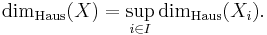
If $X=\bigcup_{i\in I}X_i$ is a finite or countable union, then

$\operatorname{dim}_{\mathrm{Haus}}(X) =\sup_{i\in I} \operatorname{dim}_{\mathrm{Haus}}(X_i).$

This can be verified directly from the definition.

If $X$ and $Y$ are metric spaces, then the Hausdorff dimension of their product satisfies

$\operatorname{dim}_{\mathrm{Haus}}(X\times Y)\ge \operatorname{dim}_{\mathrm{Haus}}(X)+ \operatorname{dim}_{\mathrm{Haus}}(Y).$

An example in which the inequality is strict has been constructed by J. M. Marstrand^[3]. It is known that when $X$ and $Y$ are Borel subsets of $\R^n$ , the Hausdorff dimension of $X\times Y$ is bounded from above by the Hausdorff dimension of $X$ plus the upper packing dimension of $Y$ . These facts are discussed in Mattila (1995).

Self-similar sets

Many sets defined by a self-similarity condition have dimensions which can be determined explicitly. Roughly, a set E is self-similar if it is the fixed point of a set-valued transformation ψ, that is ψ(E) = E, although the exact definition is given below.

Theorem. Suppose

$\psi_i: \mathbb{R}^n \rightarrow \mathbb{R}^n, \quad i=1, \ldots , m$

are contractive mappings on Rⁿ with contraction constant r_j < 1. Then there is a unique non-empty compact set A such that

$A = \bigcup_{i=1}^m \psi_i (A).$

The theorem follows from Stefan Banach's contractive mapping fixed point theorem applied to the complete metric space of non-empty compact subsets of Rⁿ with the Hausdorff distance^[4].

To determine the dimension of the self-similar set A (in certain cases), we need a technical condition called the open set condition on the sequence of contractions ψ_i which is stated as follows: There is a relatively compact open set V such that

$\bigcup_{i=1}^m\psi_i (V) \subseteq V$

where the sets in union on the left are pairwise disjoint.

Theorem. Suppose the open set condition holds and each ψ_i is a similitude, that is a composition of an isometry and a dilation around some point. Then the unique fixed point of ψ is a set whose Hausdorff dimension is s where s is the unique solution of

$\sum_{i=1}^m r_i^s = 1.$

Note that the contraction coefficient of a similitude is the magnitude of the dilation.

We can use this theorem to compute the Hausdorff dimension of the Sierpinski triangle (or sometimes called Sierpinski gasket). Consider three non-collinear points a₁, a₂, a₃ in the plane R² and let ψ_i be the dilation of ratio 1/2 around a_i. The unique non-empty fixed point of the corresponding mapping ψ is a Sierpinski gasket and the dimension s is the unique solution of

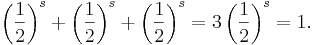
$\left(\frac{1}{2}\right)^s+\left(\frac{1}{2}\right)^s+\left(\frac{1}{2}\right)^s = 3 \left(\frac{1}{2}\right)^s =1.$

Taking natural logarithms of both sides of the above equation, we can solve for s, that is:

$s = \frac{\ln 3}{\ln 2}.$

The Sierpinski gasket is self-similar. In general a set E which is a fixed point of a mapping

$A \mapsto \psi(A) = \bigcup_{i=1}^m \psi_i(A)$

is self-similar if and only if the intersections

$H^s\left(\psi_i(E) \cap \psi_j(E)\right) =0$

where s is the Hausdorff dimension of E and $H^s$ denotes Hausdorff measure. This is clear in the case of the Sierpinski gasket (the intersections are just points), but is also true more generally:

Theorem. Under the same conditions as the previous theorem, the unique fixed point of ψ is self-similar.

Historical references

A. S. Besicovitch, On Linear Sets of Points of Fractional Dimensions, Mathematische Annalen 101 (1929).
A. S. Besicovitch and H. D. Ursell, Sets of Fractional Dimensions, Journal of the London Mathematical Society, v12 (1937). Several selections from this volume are reprinted in Classics on Fractals,ed. Gerald A. Edgar, Addison-Wesley (1993) ISBN 0-201-58701-7 See chapters 9,10,11.
F. Hausdorff, Dimension und äußeres Maß, Mathematische Annalen 79(1–2) (March 1919) pp. 157–179.

Notes

↑ Mandelbrot, Benoît (1982). The Fractal Geometry of Nature. Lecture notes in mathematics 1358. W. H. Freeman. ISBN 0716711869.
↑ M.I. Ojovan, W.E. Lee. J. Phys.: Condensed Matter, 18, 11507-11520 (2006). http://eprints.whiterose.ac.uk/1958/
↑ Marstrand, J. M. The dimension of Cartesian product sets. Proc. Cambridge Philos. Soc. 50, (1954). 198--202.
↑ K. J. Falconer, The Geometry of Fractal Sets, Cambridge University Press, 1985 Theorem 8.3

References

M. Maurice Dodson and Simon Kristensen, Hausdorff Dimension and Diophantine Approximation (June 12, 2003).
W. Hurewicz and H. Wallman, Dimension Theory, Princeton University Press, 1948.
E. Szpilrajn, La dimension et la mesure, Fundamenta Mathematica 28, 1937, pp 81-89.
Marstrand, J. M. (1954), "The dimension of cartesian product sets", Proc. Cambridge Philos. Soc. 50 (3): 198–202
Mattila, Pertti (1995), Geometry of sets and measures in Euclidean spaces, Cambridge University Press, ISBN 978-0-521-65595-8