Graph coloring

A 3-coloring suits this graph, but fewer colors would result in adjacent vertices of the same color. Finding the minimum number of colors for an arbitrary graph is NP-hard.

In graph theory, graph coloring is a special case of graph labeling; it is an assignment of labels traditionally called "colors" to elements of a graph subject to certain constraints. In its simplest form, it is a way of coloring the vertices of a graph such that no two adjacent vertices share the same color; this is called a vertex coloring. Similarly, an edge coloring assigns a color to each edge so that no two adjacent edges share the same color, and a face coloring of a planar graph assigns a color to each face or region so that no two faces that share a boundary have the same color.

Vertex coloring is the starting point of the subject, and other coloring problems can be transformed into a vertex version. For example, an edge coloring of a graph is just a vertex coloring of its line graph, and a face coloring of a planar graph is just a vertex coloring of its planar dual. However, non-vertex coloring problems are often stated and studied as is. That is partly for perspective, and partly because some problems are best studied in non-vertex form, as for instance is edge coloring.

The convention of using colors originates from coloring the countries of a map, where each face is literally colored. This was generalized to coloring the faces of a graph embedded in the plane. By planar duality it became coloring the vertices, and in this form it generalizes to all graphs. In mathematical and computer representations it is typical to use the first few positive or nonnegative integers as the "colors". In general one can use any finite set as the "color set". The nature of the coloring problem depends on the number of colors but not on what they are.

Graph coloring enjoys many practical applications as well as theoretical challenges. Beside the classical types of problems, different limitations can also be set on the graph, or on the way a color is assigned, or even on the color itself. It has even reached popularity with the general public in the form of the popular number puzzle Sudoku. Graph coloring is still a very active field of research.

Note: Many terms used in this article are defined in the glossary of graph theory.

1 History
2 Definition and terminology
3 Properties
- 3.1 Properties of the chromatic polynomial
4 Algorithms
5 Applications
6 References
7 Literature
8 See also
9 External links

History

See also: History of the four color theorem and History of graph theory

The first results about graph coloring deal almost exclusively with planar graphs in the form of the coloring of maps. While trying to color a map of the counties of England, Francis Guthrie postulated the four color conjecture, noting that four colors were sufficient to color the map so that no regions sharing a common border received the same color. Guthrie’s brother passed on the question to his mathematics teacher Augustus de Morgan at University College, who mentioned it in a letter to William Hamilton in 1852. Arthur Cayley raised the problem at a meeting of the London Mathematical Society in 1879. Over a century of failed attempts to establish the conjecture followed, until the four colour theorem was finally proved in 1976, a result that is also noteworthy for being the first major computer-aided proof.

In 1912, Birkhoff introduced the chromatic polynomial to study the coloring problems, which was generalised to the Tutte polynomial by Tutte, important structures in algebraic graph theory. Kempe had already drawn attention to the general, non-planar case in 1879^[1], and many results on generalisations of planar graph coloring to surfaces of higher order followed in the early 20th century.

In 1960, Claude Berge formulated another conjecture about graph coloring, the strong perfect graph conjecture, originally motivated by an information-theoretic concept called the zero-error capacity of a graph introduced by Shannon. The conjecture remained unresolved for 40 years, until it was established as the celebrated strong perfect graph theorem in 2002 by Chudnovsky, Robertson, Seymour, Thomas 2002.

Graph coloring has been studied as an algorithmic problem since the early 1970s. The chromatic number problem is one of Karp’s 21 NP-complete problems from 1972, around the time of various exponential-time algorithms based on backtracking and Zykov’s deletion--contraction recurrence from 1949^[2]. One of the major applications of graph coloring, register allocation in compilers was introduced in 1981.

Definition and terminology

Proper vertex coloring

The Petersen graph has chromatic number 3.

When used without any qualification, a coloring of a graph is almost always a proper vertex coloring, namely an assignment of colors to the graph’s vertices such that no two vertices sharing the same edge (graph theory) are assigned the same color. A coloring using at most k colors is called a (proper) k-coloring. A subset of vertices assigned to the same color is called a color class, every such class forms an independent set. Thus, a k-coloring is the same as a partition the vertex set into k independent sets.

The smallest number of colors needed to color a graph G is called its chromatic number, χ(G). A graph that can be assigned a (proper) k-coloring is k-colorable, and it is k-chromatic if its chromatic number is exactly k.

Chromatic polynomial

This graph can be 3-colored in 12 different ways.

The chromatic polynomial counts the number of ways a graph can be colored using no more than a given number of colors. For example, using three colors, the graph in the image to the right can be colored in 12 ways. With only two colors, it cannot be colored at all. With four colors, it can be colored in 24 + 4⋅12 = 72 ways: using all four colors, there are 4! = 24 valid colorings (every assignment of four colors to any 4-vertex graph is a proper coloring); and for every choice of three of the four colors, there are 12 valid 3-colorings. So, for the graph in the example, a table of the number of valid colorings would start like this:

Available colors	1	2	3	4	…
Number of colorings	0	0	12	72	…

The chromatic polynomial is a function $P(G,t)$ that counts the number of $t$ -colorings of $G$ . As the name indicates, for a given $G$ the function is indeed a polynomial in $t$ . For the example graph, 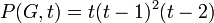$P(G,t)= t(t-1)^2(t-2)$ , and indeed $P(G,4)=72$ .

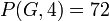The chromatic polynomial includes at least as much information about the colorability of $G$ as does the chromatic number. Indeed, χ is the smallest positive integer that is not a root of the chromatic polynomial,

$\chi (G)=\min\{ k \colon P(G,k) > 0 \}$

It was first used by Birkhoff and Lewis in their attack on the four-color theorem. They conjectured that, for a planar graph $G$ , $P(G,t)$ has no zeros in the region $[4,\infty)$ . Although it is known that such a chromatic polynomial has no zeros in the region $[5,\infty)$ and that $P(G,4) \neq 0$ . Their conjecture is still unresolved.

It remains an unsolved problem to characterize graphs which have the same chromatic polynomial and to determine precisely which polynomials are chromatic.

Chromatic polynomials for certain graphs
Triangle $K_3$	$t(t-1)(t-2)$
Complete graph $K_n$	$t(t-1)(t-2) \cdots (t-(n-1))$
Tree with $n$ vertices	$t(t-1)^{n-1}$
Cycle $C_n$	$(t-1)^n+(-1)^n(t-1)$
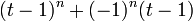Petersen graph	$t(t-1)(t-2)(t^7-12t^6+67t^5-230t^4+529t^3-814t^2+775t-352)$

Edge coloring

Main article: Edge coloring

An edge coloring of a graph, is a proper coloring of the edges, meaning an assignment of colors to edges so that no vertex is incident to two edges of the same color. An edge coloring with k colors is called a k-edge-coloring and is equivalent to the problem of partitioning the edge set into k matchings. The smallest number of colors needed for an edge coloring of a graph G is the chromatic index, or edge chromatic number, χ′(G).

Other colorings

List coloring: Each vertex chooses from a list of colors
List edge-coloring: Each edge chooses from a list of colors
Total coloring: Vertices and edges are colored
Harmonious coloring: Every pair of colors appears on at most one edge
Complete coloring: Every pair of colors appears on at least one edge
Exact coloring: Every pair of colors appears on exactly one edge
Acyclic coloring: Every 2-chromatic subgraph is acyclic
Strong coloring: Every color appears in every partition of equal size exactly once
Strong edge coloring: Edges are colored such that each color class induces a matching (equivalent to coloring the square of the line graph)
Equitable coloring: The sizes of color classes differ by at most one
Sum-coloring: The criterion of minimalization is the sum of colors
T-coloring: Distance between two colors of adjacent vertices must not belong to fixed set T
Rank coloring: If two vertices have the same color i, then every path between them contain a vertex with color greater than i
Interval edge-coloring: A color of edges meeting in a common vertex must be contiguous
Circular coloring: Motivated by task systems in which production proceeds in a cyclic way
Path coloring: Models a routing problem in graphs
Fractional coloring: Vertices may have multiple colors, and on each edge the sum of the color parts of each vertex is not greater than one
Oriented coloring: Takes into account orientation of edges of the graph
Cocoloring: An improper vertex coloring where every color class induces an independent set or a clique
Subcoloring: An improper vertex coloring where every color class induces a union of cliques
Weak coloring: An improper vertex coloring where every non-isolated node has at least one neighbor with a different color

Coloring can also be considered for signed graphs and gain graphs.

Properties

Every n-vertex graph is n-colorable, and the complete graph $K_n$ of n vertices, requires $\chi(K_n)=n$ colors.

χ(G) = 1 if and only if G is totally disconnected, i.e., it has no edges.
χ(G) ≥ 3 if and only if G has an odd cycle (equivalently, if G is not bipartite).
χ(G) ≥ ω(G), the clique number, i.e., the number of vertices of a largest clique in G.
χ(G) ≤ Δ(G) + 1, 1 more than the maximum degree of a vertex.
Brooks’s theorem^[3] states that χ(G) ≤ Δ(G) for a connected, simple graph G, unless G is a complete graph or an odd cycle
χ(G) ≤ 4, for any planar graph G. This famous result, called the four-color theorem, was stated by Augustus De Morgan in 1852, but remained unproven until 1976, when it was established by Kenneth Appel and Wolfgang Haken.

For planar graphs, vertex colorings are essentially dual to nowhere-zero flows.

About infinite graphs, much less is known. The following is one of the few results about infinite graph coloring:

If all finite subgraphs of an infinite graph G are k-colorable, then so is G. (de Bruijn and Erdős 1951)

The chromatic number of the plane, where two points are adjacent if they have unit distance, is unknown, although it is one of 4, 5, 6, or 7. Other open problems concerning the chromatic number of graphs include the Hadwiger conjecture stating that every graph with chromatic number k has a complete graph on k vertices as a minor, and the Erdős–Faber–Lovász conjecture bounding the chromatic number of unions of complete graphs that have at exactly one vertex in common to each pair.

Properties of the chromatic polynomial

$P(G,0) = 0$
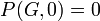
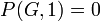$P(G,1) = 0$ if $G$ contains an edge
$P(G, t) = 0$ , if $t < \chi(G)$ .
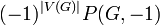$(-1)^{|V(G)|} P(G,-1)$ is the number of acyclic orientations of $G$ ^[4]
If has vertices, edges, and components …,, then
- $P(G, t)$ has degree $n$ .
- The coefficient of $t^n$ in $P(G, t)$ is 1.
- The coefficient of $t^{n-1}$ in $P(G,t)$ is $-m$ .
- The coefficients of $t^0, t^1, \dots, t^{k-1}$ are all zero.
- The coefficient of $t^k$ is nonzero.
- $P(G, t) = P(G_1, t)P(G_2,t) \cdots P(G_k,t)$
The coefficients of every chromatic polynomial alternate in signs.
A graph G with $n$ vertices is a tree if and only if $P(G, t) = t(t-1)^{n-1}$ .
The derivative evaluated at unity, $P'(G,1)$ is the chromatic invariant $\theta(G)$ up to sign

Algorithms

Graph coloring is computationally hard. It is NP-complete to decide if a given graph admits a coloring which uses at most a given number of colors. The problem remains NP-complete even on planar graphs of degree at most 4 ^[5].

Efficient algorithms

Determining if a graph can be colored with $2$ colors is equivalent to determining whether or not the graph is bipartite, and thus polynomial time-computable. As a consequence of the Strong Perfect Graph Theorem, the chromatic number of a perfect graph can be computed in polynomial time. Other classes of graphs that admit polynomial time algorithms are forests and chordal graphs.

Exact algorithms

Brute-force search for a $k$ -coloring considers every of the $\binom{n}{k}$ assignments of colors to vertices and checks for each if it is legal. To compute the chromatic number and the chromatic polynomial, this procedure is used for every $k$ , for a total running time of $O((n+1)!)$ , impractical for all but the smallest input graphs.

This can be improved based on Zykov’s identity: If $e$ is not a loop, then the chromatic number satisfies the recurrence relation:

$\chi(G) = \min \{ \, \chi(G+uv), \chi(G/uv)\,\}$

where $u$ and $v$ are nonadjecent vertices, $G+uv$ is the graph with the edge $uv$ added, and $G/uv$ is the graph where the two vertices are contracted into a single vertex.

The expressions gives rise to a recursive procedure, called the deletion–contraction algorithm. The running time satisfies the same recurrence relation as the Fibonacci numbers, so in the worst case, the algorithm runs in time within a polynomial factor of $((1+\sqrt{5})/2)^{n+m}=O(1.6180)^{n+m}$ ^[6]. The analysis can be improved to within a polynomial factor of the number $t(G)$ of spanning trees of the input graph ^[7]. In practice, branch and bound strategies and graph isomorphism rejection are employed to avoid some recursive calls, the running time depends on the heuristic used to pick the vertex pair.

Greedy coloring

The greedy algorithm considers the vertices in a specific order $v_1,\ldots, v_n$ and assigns to $v_i$ the smallest available color not used by $v_i$ ’s neighbours among $v_1,\ldots, v_{i-1}$ , adding a fresh color if needed. The quality of the resulting coloring depends on the chosen ordering. There exists an ordering that leads to a greedy coloring with the optimal number of $\chi(G)$ colors. On the other hand, greedy colorings can be arbitrarily bad; for example, there are graphs that can be 2-colored, but where there is an ordering that leads to a greedy coloring with $n/2$ colors.

If the vertices are ordered according to their degrees, the resulting greedy coloring uses at most 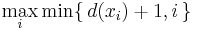$\max_i \min \{\,d(x_i ) + 1, i\,\}$ colors, at most one more than the graph’s maximum degree. This heuristic is sometimes called the Welsh–Powell algorithm^[8]. Another heuristic establishes the ordering dynamically while the algorithm proceeds, choosing next the vertex with the largest number of different colors^[9]. Many other graph coloring heuristics are similarly based on greedy coloring for a specific static or dynamic strategy of ordering the vertices, these algorithms are sometimes called sequential coloring algorithms.

Approximation

Graph coloring belongs to the hardest problems in NP in the sense that even approximating the correct answer is difficult.

The best known approximation algorithm computes a coloring of size at most within a factor $O(n(\log n)^{-3}(\log\log n)^2)$ of the chromatic number.^[10] For all $\epsilon>0$ it is NP-hard to approximate the chromatic number within $n^{1-\epsilon}$ ^[11]

Computing the chromatic polynomial

Other algorithms are known, but all are exponential in the size of the graph. In general, computing the chromatic polynomial is #P-complete, so it is unlikely that a polynomial time algorithm for all graphs will be found.

Applications

The problem of coloring a graph has found a number of applications. Some of them are scheduling, register allocation in compilers, bandwidth allocation, and pattern matching.

The recreational puzzle Sudoku can be seen as completing a 9-coloring on given specific graph with 81 vertices.

References

↑ Jensen and Toft, p. 2
↑ Zykov, 1949
↑ Brooks, R. L. On Coloring the Nodes of a Network. Proc. Cambridge Philos. Soc. 37, 194-197, 1941.
↑ Stanley, 1973
↑ M. R. Garey, D. S. Johnson, and L. Stockmeyer. Some simplified NP-complete problems. Proceedings of the sixth annual ACM symposium on Theory of computing, p.47-63. 1974.
↑ H. S. Wilf, Algorithms and Complexity, Prentice–Hall, 1986.
↑ K. Sekine, H. Imai, S. Tani, Computing the Tutte polynomial of a graph of moderate size, Algorithms and Computation, 6th International Symposium (ISAAC ’95), Cairns, Australia, December 4–6, 1995, Lecture Notes in Computer Science 1004, Springer, 1995, pp. 224–233.
↑ D. J. A. Welsh and M. B. Powell (1967). "An upper bound for the chromatic number of a graph and its application to timetabling problems". The Computer Journal 10 (1): 85–86. doi:10.1093/comjnl/10.1.85.
↑ Brèlaz, D., New methods to color the vertices of a graph, Communica- tions of the Assoc. of Comput. Machinery 22 (1979), 251-256.
↑ Halldórsson, M. M., 1993, A still better performance guarantee for approximate graph coloring, Inform. Process. Lett. 45, 19-23.
↑ D. Zuckerman. Linear degree extractors and the inapproximability of Max Clique and Chromatic Number. Theory of Computing, 3:103–128, 2007.

Literature

R. L. Brooks (1941). "On colouring the nodes of a network". Proc. Cambridge Phil. Soc. 37: 194–197.
N. G. de Bruijn; P. Erdős (1951), "A colour problem for infinite graphs and a problem in the theory of relations", Nederl. Akad. Wetensch. Proc. Ser. A 54: 371–373 (= Indag. Math. 13)
Tommy R. Jensen and Bjarne Toft (1995), Graph Coloring Problems, Wiley-Interscience, New York, ISBN 0-471-02865-7
Marek Kubale et al. (2004). Graph Colorings. American Mathematical Society. ISBN 0-8218-3458-4.
Michael R. Garey, David S. Johnson, and L. Stockmeyer (1974). "Some simplified NP-complete problems". Proceedings of the sixth annual ACM symposium on Theory of computing: 47-63.
Michael R. Garey and David S. Johnson (1979). Computers and Intractability: A Guide to the Theory of NP-Completeness. W.H. Freeman. ISBN 0-7167-1045-5. A1.1: GT4, pg.191.
West, Douglas B. (1996). Introduction to Graph Theory. Prentice-Hall. ISBN 0-13-227828-6.
A. A. Zykov (1949). "On some properties of linear complexes (in Russian)". Math. Sbornik. 24: 163-188.

External links

Graph Coloring Page by Joseph Culberson (graph coloring programs)
CoLoRaTiOn by Jim Andrews and Mike Fellows is a graph coloring puzzle
GF-Graph Coloring Program [1]
Links to Graph Coloring source codes
Code for efficiently computing Tutte, Chromatic and Flow Polynomials by Gary Haggard, David J. Pearce and Gordon Royle: [2]