Gini coefficient

(The area of the whole triangle is defined as 1, not 0.5)
The Gini coefficient is a measure of statistical dispersion most prominently used as a measure of inequality of income distribution or inequality of wealth distribution. It is defined as a ratio with values between 0 and 1: A low Gini coefficient indicates more equal income or wealth distribution, while a high Gini coefficient indicates more unequal distribution. 0 corresponds to perfect equality (everyone having exactly the same income) and 1 corresponds to perfect inequality (where one person has all the income, while everyone else has zero income). The Gini coefficient requires that no one have a negative net income or wealth. Worldwide, Gini coefficients range from approximately 0.232 in Denmark to 0.707 in Namibia. Most free market nations have a Gini coeffient between.25 and.50.
The Gini index is the Gini coefficient expressed as a percentage, thus Denmark's Gini index is 23.2% (Mathematically, this is equal to the Gini coefficient of 0.232, but the percentage sign is often omitted in the Gini index.)
The Gini coefficient was developed by the Italian statistician Corrado Gini and published in his 1912 paper "Variability and Mutability" (Italian: Variabilità e mutabilità ).
Calculation
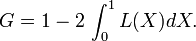
The Gini coefficient is defined as a ratio of the areas on the Lorenz curve diagram. If the area between the line of perfect equality and Lorenz curve is A, and the area under the Lorenz curve is B, then the Gini coefficient is A/(A+B). Since A+B = 0.5, the Gini coefficient, G = A/(0.5) = 2A = 1-2B. If the Lorenz curve is represented by the function Y = L(X), the value of B can be found with integration and:
In some cases, this equation can be applied to calculate the Gini coefficient without direct reference to the Lorenz curve. For example:
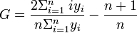
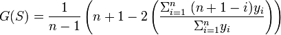
- For a population uniform on the values yi, i = 1 to n, indexed in non-decreasing order ( yi ≤ yi+1):
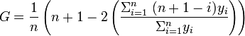
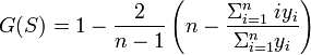
- This may be simplified to:
- For a discrete probability function f(y), where yi, i = 1 to n, are the points with nonzero probabilities and which are indexed in increasing order ( yi < yi+1):
- where
 and
and 
- For a cumulative distribution function F(y) that is piecewise differentiable, has a mean μ, and is zero for all negative values of y:

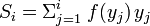
- Since the Gini coefficient is half the relative mean difference, it can also be calculated using formulas for the relative mean difference. For a random sample S consisting of values yi, i = 1 to n, that are indexed in non-decreasing order ( yi ≤ yi+1), the statistic:
- is a consistent estimator of the population Gini coefficient, but is not, in general, unbiased. Like, G, G(S) has a simpler form:
 .
.
There does not exist a sample statistic that is in general an unbiased estimator of the population Gini coefficient, like the relative mean difference.
Sometimes the entire Lorenz curve is not known, and only values at certain intervals are given. In that case, the Gini coefficient can be approximated by using various techniques for interpolating the missing values of the Lorenz curve. If ( X k , Yk ) are the known points on the Lorenz curve, with the X k indexed in increasing order ( X k - 1 < X k ), so that:
- Xk is the cumulated proportion of the population variable, for k = 0,...,n, with X0 = 0, Xn = 1.
- Yk is the cumulated proportion of the income variable, for k = 0,...,n, with Y0 = 0, Yn = 1.
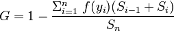
If the Lorenz curve is approximated on each interval as a line between consecutive points, then the area B can be approximated with trapezoids and:
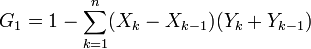
is the resulting approximation for G. More accurate results can be obtained using other methods to approximate the area B, such as approximating the Lorenz curve with a quadratic function across pairs of intervals, or building an appropriately smooth approximation to the underlying distribution function that matches the known data. If the population mean and boundary values for each interval are also known, these can also often be used to improve the accuracy of the approximation.
The Gini coefficient calculated from a sample is a statistic and its standard error, or confidence intervals for the population Gini coefficient, should be reported. These can be calculated using bootstrap techniques but those proposed have been mathematically complicated and computationally onerous even in an era of fast computers. Ogwang (2000) made the process more efficient by setting up a “trick regression model” in which the incomes in the sample are ranked with the lowest income being allocated rank 1. The model then expresses the rank (dependent variable) as the sum of a constant A and a normal error term whose variance is inversely proportional to yk;
Ogwang showed that G can be expressed as a function of the weighted least squares estimate of the constant A and that this can be used to speed up the calculaton of the jackknife esimate for the standard error. Giles (2004) argued that the standard error of the estimate of A can be used to derive that of the estimate of G directly without using a jackknife at all. However it has since been argued that this is dependent on the model’s assumptions about the error distributions (Ogwang 2004) and the independence of error terms (Reza & Gastwirth 2006) and that these assumptions are often not valid for real data sets. It may therefore be better to stick with jackknife methods such as those proposed by Yitzhaki (1991) and Karagiannis and Kovacevic (2000). The debate continues.
The gini coefficient can be calculated if you know the mean of a distribution, the number of people (or percentiles), and the income of each person (or percentile). Princeton development economist Angus Deaton (1997, 139) has simplified the Gini calculation to one easy formula:
where u is mean income of the population, Pi is the income rank P of person i, with income X, such that the richest person receives a rank of 1 and the poorest a rank of N. This effectively gives higher weight to poorer people in the income distribution, which allows the Gini to meet the Transfer Principle.
Income Gini indices in the world
A complete listing is in list of countries by income equality; the article economic inequality discusses the social and policy aspects of income and asset inequality.

While most developed European nations tend to have Gini indices between 24 and 36, the United States' and Mexico's Gini indices are both above 40, indicating that the United States and Mexico have greater inequality. Using the Gini can help quantify differences in welfare and compensation policies and philosophies. However it should be borne in mind that the Gini coefficient can be misleading when used to make political comparisons between large and small countries (see criticisms section).
The Gini index for the entire world has been estimated by various parties to be between 56 and 66.[1][2]

Correlation with per-capita GDP
Poor countries (those with low per-capita GDP) generally have higher Gini indices, spread between 40 and 65, with extremes at 25 and 71, while rich countries generally have lower Gini indices (under 40). The lowest Gini coefficients (under 30) can be found in continental Europe. Overall, there is a clear negative correlation between Gini coefficient and GDP per capita, the U.S.A, Hongkong and Singapore being rich exceptions with high Gini coefficients.
In many of the former socialist countries and in-development capitalist countries (e.g., Brazil), the sizeable underground economy may hide income for many. In such a case, earning/wealth statistics over-represent certain income ranges (i.e., in lower-income regions), and may alter the Gini coefficient either up or down.
US income Gini indices over time
Gini indices for the United States at various times, according to the US Census Bureau:
- 1929: 45.0 (estimated)
- 1947: 37.6 (estimated)
- 1967: 39.7 (first year reported)
- 1968: 38.6 (lowest index reported)
- 1970: 39.4
- 1980: 40.3
- 1990: 42.8
- 2000: 46.2
- 2005: 46.9
- 2006: 47.0 (highest index reported)
- 2007: 46.3 [3]
Note: Estimates are not 100% accurate.
Advantages of Gini coefficient as a measure of inequality
- The Gini coefficient's main advantage is that it is a measure of inequality by means of a ratio analysis, rather than a variable unrepresentative of most of the population, such as per capita income or gross domestic product.
- It can be used to compare income distributions across different population sectors as well as countries, for example the Gini coefficient for urban areas differs from that of rural areas in many countries (though the United States' urban and rural Gini coefficients are nearly identical).
- It is sufficiently simple that it can be compared across countries and be easily interpreted. GDP statistics are often criticised as they do not represent changes for the whole population; the Gini coefficient demonstrates how income has changed for poor and rich. If the Gini coefficient is rising as well as GDP, poverty may not be improving for the majority of the population.
- The Gini coefficient can be used to indicate how the distribution of income has changed within a country over a period of time, thus it is possible to see if inequality is increasing or decreasing.
- The Gini coefficient satisfies four important principles:
- Anonymity: it does not matter who the high and low earners are.
- Scale independence: the Gini coefficient does not consider the size of the economy, the way it is measured, or whether it is a rich or poor country on average.
- Population independence: it does not matter how large the population of the country is.
- Transfer principle: if income (less than the difference), is transferred from a rich person to a poor person the resulting distribution is more equal.
Disadvantages of Gini coefficient as a measure of inequality
- The Gini coefficient of different sets of people cannot be averaged to obtain the Gini coefficient of all the people in the sets: if a Gini coefficient were to be calculated for each person it would always be zero. For a large, economically diverse country, a much higher coefficient will be calculated for the country as a whole than will be calculated for each of its regions. (The coefficient is usually applied to measurable nominal income rather than local purchasing power, tending to increase the calculated coefficient across larger areas.)
- For this reason, the scores calculated for individual countries within the EU are difficult to compare with the score of the entire US: the overall value for the EU should be used in that case, 31.3[4], which is still much lower than the United States', 45.[5] Using decomposable inequality measures (e.g. the Theil index
 converted by
  into a inequality coefficient) averts such problems.
- The Lorenz curve may understate the actual amount of inequality if richer households are able to use income more efficiently than lower income households. From another point of view, measured inequality may be the result of more or less efficient use of household incomes.
- Economies with similar incomes and Gini coefficients can still have very different income distributions. This is because the Lorenz curves can have different shapes and yet still yield the same Gini coefficient.
- It measures current income rather than lifetime income. A society in which everyone earned the same over a lifetime would appear unequal because of people at different stages in their life; a society in which students study rather than save can never have a coefficient of 0. However, Gini coefficient can also be calculated for any kind of distribution, e.g. for wealth. [6]
Problems in using the Gini coefficient
- Gini coefficients do include income gained from wealth; however, the Gini coefficient is used to measure net income more than net worth, which can be misinterpreted. For example, Sweden has a low Gini coefficient for income distribution and a higher Gini coefficient for wealth (the wealth inequality is low by international standards, but still significant: 5% of Swedish household shareholders hold 77% of the share value owned by households)[7]. In other words, the Gini income coefficient should not be interpreted as measuring effective egalitarianism. Distribution of stock ownership does not appear to correlate to many recognized indicators of egalitarianism.
- Too often only the Gini coefficient is quoted without describing the proportions of the quantiles used for measurement. As with other inequality coefficients, the Gini coefficient is influenced by the granularity of the measurements. For example, five 20% quantiles (low granularity) will usually yield a lower Gini coefficient than twenty 5% quantiles (high granularity) taken from the same distribution. This is an often encountered problem with measurements.
- Care should be taken in using the Gini coefficient as a measure of egalitarianism, as it is properly a measure of income dispersion. Two equally egalitarian countries with different immigration policies may have different Gini coefficients.
- The Gini coefficient is generally measured at a point in time, hence it potentially misses a lot of dynamic information about individual's lifetime income. Other factors, such as age distribution within a population and mobility within income classes are ignored. It is possible for a given economy to have a higher Gini coefficient at any one point in time than another economy, while the Gini coefficient calculated over individuals' lifetime income is actually lower than the "more equal" (at a given point in time) economy's. Essentially, what matter is not just inequality in any particular year, but the composition of the distribution over time.
General problems of measurement
- Comparing income distributions among countries may be difficult because benefits systems may differ. For example, some countries give benefits in the form of money while others give food stamps, which might not be counted by some economists and researchers as income in the Lorenz curve and therefore not taken into account in the Gini coefficient. The USA counts income before benefits, while France counts it after benefits, making the USA appear more unequal vis-a-vis France than it is.
- The measure will give different results when applied to individuals instead of households. When different populations are not measured with consistent definitions, comparison is not meaningful.
- As for all statistics, there may be systematic and random errors in the data. The meaning of the Gini coefficient decreases as the data become less accurate. Also, countries may collect data differently, making it difficult to compare statistics between countries.
As one result of this criticism, in addition to or in competition with the Gini coefficient entropy measures are frequently used (e.g. the Theil Index and the index of Atkinson). These measures attempt to compare the distribution of resources by intelligent agents in the market with a maximum entropy random distribution, which would occur if these agents acted like non-intelligent particles in a closed system following the laws of statistical physics.
Credit risk
The Gini coefficient is also commonly used for the measurement of the discriminatory power of rating systems in credit risk management. Since Gini coefficient addresses wealth inequality it may be important to understand what a transformative asset is. Transformative assets increase the Gini coefficient as they provide a family or individual with a wealth advantage over most persons.
The discriminatory power refers to a credit risk model's ability to differentiate between defaulting and non-defaulting clients. The above formula  may be used for the final model and also at individual model factor level, to quantify the discriminatory power of individual factors. In this case, negative Gini Coefficient values are possible. This is as a result of too many non defaulting clients falling into the lower points scale e.g. factor has a 10 point scale and 30% of non defaulting clients are being assigned the lowest points available e.g. 0 or negative points. This indicates that the factor is behaving in a counter-intuitive manner and would require further investigation at the model development stage.
References: The Analytics of risk model validation
See also
|
|
|
References
- ↑ Bob Sutcliffe (April 2007), Postscript to the article ‘World inequality and globalization’ (Oxford Review of Economic Policy, Spring 2004), http://siteresources.worldbank.org/INTDECINEQ/Resources/PSBSutcliffe.pdf, retrieved on 2007-12-13
- ↑ United Nations Development Programme
- ↑ Note that the calculation of the index for the United States was changed in 1992, resulting in an upwards shift of about 2.
- ↑ European Union, CIA World Factbook, https://www.cia.gov/library/publications/the-world-factbook/geos/ee.html, retrieved on 2007-12-13
- ↑ United States, CIA World Factbook, https://www.cia.gov/library/publications/the-world-factbook/geos/us.html, retrieved on 2007-12-13
- ↑ Friedman, David D.
- ↑ (Data from the Statistics Sweden.)
Further reading
- Amiel, Y.; Cowell, F.A. (1999). Thinking about Inequality. Cambridge.
- Anand, Sudhir (1983). Inequality and Poverty in Malaysia. New York: Oxford University Press.
- Brown, Malcolm (1994). "Using Gini-Style Indices to Evaluate the Spatial Patterns of Health Practitioners: Theoretical Considerations and an Application Based on Alberta Data". Social Science Medicine 38: 1243–1256. doi:.
- Chakravarty, S. R. (1990). Ethical Social Index Numbers. New York: Springer-Verlag.
- Deaton, Angus (1997). Analysis of Household Surveys. Baltimore MD: Johns Hopkins University Press.
- Dixon, PM, Weiner J., Mitchell-Olds T, Woodley R. (1987). "Bootstrapping the Gini coefficient of inequality". Ecology 68: 1548–1551. doi:.
- Dorfman, Robert (1979). "A Formula for the Gini Coefficient". The Review of Economics and Statistics 61: 146–149. doi:.
- Gastwirth, Joseph L. (1972). "The Estimation of the Lorenz Curve and Gini Index". The Review of Economics and Statistics 54: 306–316. doi:.
- Giles, David (2004). "Calculating a Standard Error for the Gini Coefficient: Some Further Results". Oxford Bulletin of Economics and Statistics 66: 425–433. doi:.
- Gini, Corrado (1912). "Variabilità e mutabilità" Reprinted in Memorie di metodologica statistica (Ed. Pizetti E, Salvemini, T). Rome: Libreria Eredi Virgilio Veschi (1955).
- Gini, Corrado (1921). "Measurement of Inequality and Incomes". The Economic Journal 31: 124–126. doi:.
- Karagiannis, E. and Kovacevic, M. (2000). "A Method to Calculate the Jackknife Variance Estimator for the Gini Coefficient". Oxford Bulletin of Economics and Statistics 62: 119–122. doi:.
- Mills, Jeffrey A.; Zandvakili, Sourushe (1997). "Statistical Inference via Bootstrapping for Measures of Inequality". Journal of Applied Econometrics 12: 133–150. doi:.
- Modarres, Reza and Gastwirth, Joseph L. (2006). "A Cautionary Note on Estimating the Standard Error of the Gini Index of Inequality". Oxford Bulletin of Economics and Statistics 68: 385–390. doi:.
- Morgan, James (1962). "The Anatomy of Income Distribution". The Review of Economics and Statistics 44: 270–283. doi:.
- Ogwang, Tomson (2000). "A Convenient Method of Computing the Gini Index and its Standard Error". Oxford Bulletin of Economics and Statistics 62: 123–129. doi:.
- Ogwang, Tomson (2004). "Calculating a Standard Error for the Gini Coefficient: Some Further Results: Reply". Oxford Bulletin of Economics and Statistics 66: 435–437. doi:.
- Xu, Kuan (January, 2004). "How Has the Literature on Gini's Index Evolved in the Past 80 Years?". Department of Economics, Dalhousie University. Retrieved on 2006-06-01. The Chinese version of this paper appears in Xu, Kuan (2003). "How Has the Literature on Gini's Index Evolved in the Past 80 Years?". China Economic Quarterly 2: 757–778.
- Yitzhaki, S. (1991). "Calculating Jackknife Variance Estimators for Parameters of the Gini Method". Journal of Business and Economic Statistics 9: 235–239. doi:.
External links
- The World Bank: Measuring Inequality
- United States Census Bureau List of Gini Coefficients by State for Families and Households
- Gini index calculated for all countries (from internet archive)
- Comparison of Urban and Rural Areas' Gini Coefficients Within States
- World Income Inequality Database
- Forbes Article, In praise of inequality
- Travis Hale, University of Texas Inequality Project: The Theoretical Basics of Popular Inequality Measures, online computation of examples: 1A, 1B
- An application of the Gini coefficient to software : Measuring Software Project Risk With The Gini Coefficient
- Deutsche Bundesbank: Do banks diversify loan portfolios?, 2005 (on using e.g. the Gini coefficient for risc evaluation of loan portefolios)
- Software:
- Free Online Calculator computes the Gini Coefficient, plots the Lorenz curve, and computes many other measures of concentration for any dataset
- Free Calculator: Online and downloadable scripts (Python and Lua) for Atkinson, Gini, and Hoover inequalities
- Users of the R data analysis software can install the "ineq" package which allows for computation of a variety of inequality indices including Gini, Atkinson, Theil.
- A MATLAB Inequality Package, including code for computing Gini, Atkinson, Theil indexes and for plotting the Lorenz Curve. Many examples are available.