Fundamental theorem of calculus
| Topics in calculus |
|
Fundamental theorem |
| Differentiation |
|
Product rule |
| Integration |
|
Lists of integrals |
The fundamental theorem of calculus specifies the relationship between the two central operations of calculus, differentiation and integration.
The first part of the theorem, sometimes called the first fundamental theorem of calculus, shows that an indefinite integration[1] can be reversed by a differentiation.
The second part, sometimes called the second fundamental theorem of calculus, allows one to compute the definite integral of a function by using any one of its infinitely many antiderivatives. This part of the theorem has invaluable practical applications, because it markedly simplifies the computation of definite integrals.
The first published statement and proof of a restricted version of the fundamental theorem was by James Gregory (1638-1675)[2]. Isaac Barrow proved the first completely general version of the theorem, while Barrow's student Isaac Newton (1643–1727) completed the development of the surrounding mathematical theory. Gottfried Leibniz (1646–1716) systematized the knowledge into a calculus for infinitesimal quantities.
The Fundamental Theorem of Calculus is sometimes also called Leibniz's Fundamental Theorem of Calculus or the Torricelli–Barrow theorem.
Contents |
Physical intuition
Intuitively, the theorem simply states that the sum of infinitesimal changes in a quantity over time (or some other quantity) add up to the net change in the quantity.
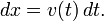
To comprehend this statement, we will start with an example. Suppose a particle travels in a straight line with its position, x, given by x(t) where t is time and x(t) means that x is a function of t. The derivative of this function is equal to the infinitesimal change in quantity, dx, per infinitesimal change in time, dt (of course, the derivative itself is dependent on time). Let us define this change in distance per change in time as the velocity v of the particle. In Leibniz's notation:

Rearranging this equation, it follows that:
By the logic above, a change in x (or Δx) is the sum of the infinitesimal changes dx. It is also equal to the sum of the infinitesimal products of the derivative and time. This infinite summation is integration; hence, the integration operation allows the recovery of the original function from its derivative. As one can reasonably infer, this operation works in reverse as we can differentiate the result of our integral to recover the original derivative.
Geometric intuition

Suppose we are given a smooth continuous function y = ƒ(x), and have plotted its graph as a curve. Then for each value of x, intuitively it makes sense that there is a corresponding area function A(x), representing the area beneath the curve between 0 and x. We may not know a "formula" for the function A(x), but intuitively we understand that it is simply the area under the curve.
Now suppose we wanted to compute the area under the curve between x and x+h. We could compute this area by finding the area between 0 and x+h, then subtracting the area between 0 and x. In other words, the area of this “sliver” would be A(x+h) − A(x).
There is another way to estimate the area of this same sliver. Multiply h by ƒ(x) to find the area of a rectangle that is approximately the same size as this sliver. In fact, it makes intuitive sense that for very small values of h, the approximation will become very good.
At this point we know that A(x+h) − A(x) is approximately equal to ƒ(x)·h, and we intuitively understand that this approximation becomes better as h grows smaller. In other words, ƒ(x)·h ≈ A(x+h) − A(x), with this approximation becoming an equality as h approaches 0 in the limit.
Divide both sides of this equation by h. Then we have

As h approaches 0, we recognized that the right hand side of this equation is simply the derivative A’(x) of the area function A(x). The left-hand side of the equation simply remains ƒ(x), since no h is present.
We have shown informally that ƒ(x) = A’(x). In other words, the derivative of the area function A(x) is the original function ƒ(x). Or, to put it another way, the area function is simply the antiderivative of the original function.
What we have shown is that, intuitively, computing the derivative of a function and “finding the area” under its curve are "opposite" operations. This is the crux of the Fundamental Theorem of Calculus. The bulk of the theorem's proof is devoted to showing that the area function A(x) exists in the first place.
Formal statements
There are two parts to the Fundamental Theorem of Calculus. Loosely put, the first part deals with the derivative of an antiderivative, while the second part deals with the relationship between antiderivatives and definite integrals.
First part
This part is sometimes referred to as the First Fundamental Theorem of Calculus.[3]
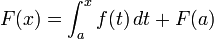
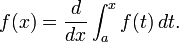
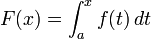
Let f be a continuous real-valued function defined on a closed interval [a, b]. Let F be the function defined, for all x in [a, b], by

Then, F is continuous on [a, b], differentiable on the open interval (a, b), and
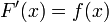
for all x in (a, b).
Second part
This part is sometimes referred to as the Second Fundamental Theorem of Calculus.[4]
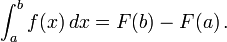
Let f be a continuous real-valued function defined on a closed interval [a, b]. Let F be an antiderivative of f, that is one of the infinitely many functions such that, for all x in [a, b],

Then
Corollary
Let f be a continuous real-valued function defined on a closed interval [a, b]. Let F be a function such that, for all x in [a, b],
Then, for all x in [a, b],
and
Examples
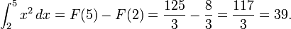
As an example, suppose you need to calculate

Here,  and we can use
  as the antiderivative. Therefore:
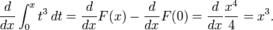
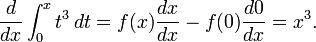
Or, more generally, suppose you need to calculate

Here,  and we can use
  as the antiderivative. Therefore:
But this result could have been found much more easily as
Proof of the First Part
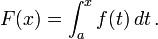
For a given f(t), define the function F(x) as
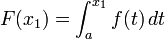
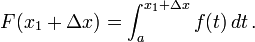
For any two numbers x1 and x1 + Δx in [a, b], we have
and
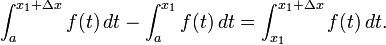
Subtracting the two equations gives

It can be shown that
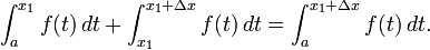
- (The sum of the areas of two adjacent regions is equal to the area of both regions combined.)
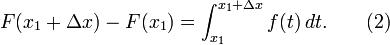
Manipulating this equation gives
Substituting the above into (1) results in
According to the mean value theorem for integration, there exists a c in [x1, x1 + Δx] such that
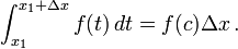
Substituting the above into (2) we get

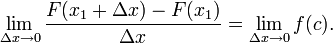
Dividing both sides by Δx gives
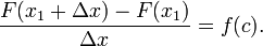
- Notice that the expression on the left side of the equation is Newton's difference quotient for F at x1.
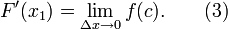
Take the limit as Δx → 0 on both sides of the equation.
The expression on the left side of the equation is the definition of the derivative of F at x1.
To find the other limit, we will use the squeeze theorem. The number c is in the interval [x1, x1 + Δx], so x1 ≤ c ≤ x1 + Δx.
Also,  and
and 
Therefore, according to the squeeze theorem,

Substituting into (3), we get

The function f is continuous at c, so the limit can be taken inside the function. Therefore, we get
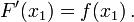
which completes the proof.
(Leithold et al, 1996)
Proof of the Second Part
This is a limit proof by Riemann sums.
Let f be continuous on the interval [a, b], and let F be an antiderivative of f. Begin with the quantity
Let there be numbers
- x1, ..., xn
such that

It follows that

Now, we add each F(xi) along with its additive inverse, so that the resulting quantity is equal:
![\begin{matrix} F(b) - F(a) & = & F(x_n)\,+\,[-F(x_{n-1})\,+\,F(x_{n-1})]\,+\,\ldots\,+\,[-F(x_1) + F(x_1)]\,-\,F(x_0) \, \\
& = & [F(x_n)\,-\,F(x_{n-1})]\,+\,[F(x_{n-1})\,+\,\ldots\,-\,F(x_1)]\,+\,[F(x_1)\,-\,F(x_0)] \,. \end{matrix}](/2009-wikipedia_en_wp1-0.7_2009-05/I/bde262027624d2d1b7d79d67751f9444.png)
The above quantity can be written as the following sum:
![F(b) - F(a) = \sum_{i=1}^n \,[F(x_i) - F(x_{i-1})]\,. \qquad (1)](/2009-wikipedia_en_wp1-0.7_2009-05/I/5fbb95b91da8e3ddceb869337d7323d5.png)
Next we will employ the mean value theorem. Stated briefly,
Let F be continuous on the closed interval [a, b] and differentiable on the open interval (a, b). Then there exists some c in (a, b) such that
It follows that

The function F is differentiable on the interval [a, b]; therefore, it is also differentiable and continuous on each interval xi-1. Therefore, according to the mean value theorem (above),

Substituting the above into (1), we get
![F(b) - F(a) = \sum_{i=1}^n \,[F'(c_i)(x_i - x_{i-1})]\,.](/2009-wikipedia_en_wp1-0.7_2009-05/I/9a27d0ce017fd6a29ffc33d230617973.png)
The assumption implies  Also,
Also,  can be expressed as
  of partition
  .
.
![F(b) - F(a) = \sum_{i=1}^n \,[f(c_i)(\Delta x_i)]\,. \qquad (2)](/2009-wikipedia_en_wp1-0.7_2009-05/I/2371fea52b0fcdf7735b3d7eb5c7ef11.png)

Notice that we are describing the area of a rectangle, with the width times the height, and we are adding the areas together. Each rectangle, by virtue of the Mean Value Theorem, describes an approximation of the curve section it is drawn over. Also notice that  does not need to be the same for any value of , or in other words that the width of the rectangles can differ. What we have to do is approximate the curve with
  rectangles. Now, as the size of the partitions get smaller and n increases, resulting in more partitions to cover the space, we will get closer and closer to the actual area of the curve.
By taking the limit of the expression as the norm of the partitions approaches zero, we arrive at the Riemann integral. That is, we take the limit as the largest of the partitions approaches zero in size, so that all other partitions are smaller and the number of partitions approaches infinity.
So, we take the limit on both sides of (2). This gives us
![\lim_{\| \Delta \| \to 0} F(b) - F(a) = \lim_{\| \Delta \| \to 0} \sum_{i=1}^n \,[f(c_i)(\Delta x_i)]\,.](/2009-wikipedia_en_wp1-0.7_2009-05/I/291ffe044566ee45e9edf75a078f0a9e.png)
Neither F(b) nor F(a) is dependent on ||Δ||, so the limit on the left side remains F(b) - F(a).
![F(b) - F(a) = \lim_{\| \Delta \| \to 0} \sum_{i=1}^n \,[f(c_i)(\Delta x_i)]\,.](/2009-wikipedia_en_wp1-0.7_2009-05/I/c57e85d849c57c1ebd9f8c17a575c57b.png)
The expression on the right side of the equation defines an integral over f from a to b. Therefore, we obtain
which completes the proof.
Generalizations
We don't need to assume continuity of f on the whole interval. Part I of the theorem then says: if f is any Lebesgue integrable function on [a, b] and x0 is a number in [a, b] such that f is continuous at x0, then
is differentiable for x = x0 with F'(x0) = f(x0). We can relax the conditions on f still further and suppose that it is merely locally integrable. In that case, we can conclude that the function F is differentiable almost everywhere and F'(x) = f(x) almost everywhere. This is sometimes known as Lebesgue's differentiation theorem.
Part II of the theorem is true for any Lebesgue integrable function f which has an antiderivative F (not all integrable functions do, though).
The version of Taylor's theorem which expresses the error term as an integral can be seen as a generalization of the Fundamental Theorem.
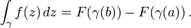
There is a version of the theorem for complex functions: suppose U is an open set in C and f: U → C is a function which has a holomorphic antiderivative F on U. Then for every curve γ: [a, b] → U, the curve integral can be computed as
The fundamental theorem can be generalized to curve and surface integrals in higher dimensions and on manifolds.
One of the most powerful statements in this direction is Stokes' theorem: Let M be an oriented piecewise smooth manifold of dimension n and let  be an n−1 form that is a compactly supported differential form on M of class C1. If ∂M denotes the boundary of M with its induced orientation, then
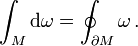
Here  is the exterior derivative, which is defined using the manifold structure only.
The theorem is often used in situations where M is an embedded oriented submanifold of some bigger manifold on which the form is defined.
See also
- Differintegral
Notes
- ↑ More exactly, the theorem deals with definite integration with variable upper limit and arbitrarily selected lower limit. This particular kind of definite integration allows us to compute one of the infinitely many antiderivatives of a function (except for those which do not have a zero). Hence, it is almost equivalent to indefinite integration, defined by most authors as an operation which yields any one of the possible antiderivatives of a function, including those without a zero.
- ↑ See, e.g., Marlow Anderson, Victor J. Katz, Robin J. Wilson, Sherlock Holmes in Babylon and Other Tales of Mathematical History, Mathematical Association of America, 2004, p. 114.
- ↑ Apostol 1967, §5.1
- ↑ Apostol 1967, §5.3
References
- Apostol, Tom M. (1967), Calculus, Vol. 1: One-Variable Calculus with an Introduction to Linear Algebra (2nd ed.), New York: John Wiley & Sons, ISBN 978-0-471-00005-1.
- Larson, Ron; Edwards, Bruce H.; Heyd, David E. (2002), Calculus of a single variable (7th ed.), Boston: Houghton Mifflin Company.
- Leithold, L. (1996), The calculus of a single variable (6th ed.), New York: HarperCollins College Publishers.
- Malet, A, Studies on James Gregorie (1638-1675) (PhD Thesis, Princeton, 1989).
- Stewart, J. (2003), Calculus: early transcendentals, Belmont, California: Thomson/Brooks/Cole.
- Turnbull, H. W., ed. (1939), The James Gregory Tercentenary Memorial Volume, London.