Fourier series
| Fourier transforms |
|---|
| Continuous Fourier transform |
| Fourier series |
| Discrete Fourier transform |
| Discrete-time Fourier transform |
|
|
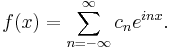
In mathematics, a Fourier series decomposes a periodic function into a sum of simple oscillating functions, namely sines and cosines. The study of Fourier series is a branch of Fourier analysis. Fourier series were introduced by Joseph Fourier (1768–1830) for the purpose of solving the heat equation in a metal plate. It led to a revolution in mathematics, forcing mathematicians to reexamine the foundations of mathematics and leading to many modern theories such as Lebesgue integration.
The heat equation is a partial differential equation. Prior to Fourier's work, there was no known solution to the heat equation in a general situation, although particular solutions were known if the heat source behaved in a simple way, in particular, if the heat source was a sine or cosine wave. These simple solutions are now sometimes called eigensolutions. Fourier's idea was to model a complicated heat source as a superposition (or linear combination) of simple sine and cosine waves, and to write the solution as a superposition of the corresponding eigensolutions. This superposition or linear combination is called the Fourier series.
Although the original motivation was to solve the heat equation, it later became obvious that the same techniques could be applied to a wide array of mathematical and physical problems. The basic results are very easy to understand using the modern theory.
The Fourier series has many applications in electrical engineering, vibration analysis, acoustics, optics, signal processing, image processing, quantum mechanics, etc.
Contents |
Historical development
Fourier series are named in honor of Joseph Fourier (1768-1830), who made important contributions to the study of trigonometric series, after preliminary investigations by Leonhard Euler, Jean le Rond d'Alembert, and Daniel Bernoulli. He applied this technique to find the solution of the heat equation, publishing his initial results in 1807 and 1811, and publishing his Théorie analytique de la chaleur in 1822.
From a modern point of view, Fourier's results are somewhat informal, due to the lack of a precise notion of function and integral in the early nineteenth century. Later, Dirichlet and Riemann expressed Fourier's results with greater precision and formality.
A revolutionary article
| “ | 
Multiplying both sides by
|
” |
|
—Joseph Fourier, Mémoire sur la propagation de la chaleur dans les corps solides, pp. 218--219.[1] |
||
 , and then integrating from
  to
to  yields:
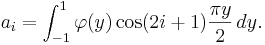
In these few lines, which are surprisingly close to the modern formalism used in Fourier series, Fourier unwittingly revolutionized both mathematics and physics. Although similar trigonometric series were previously used by Euler, d'Alembert, Daniel Bernoulli and Gauss, Fourier believed that such trigonometric series could represent arbitrary functions. While this is not true, the attempts over many years to clarify this idea have led to important discoveries in the theories of convergence, function spaces, and harmonic analysis.
When Fourier submitted his paper in 1807, the committee (composed of no lesser mathematicians than Lagrange, Laplace, Malus and Legendre, among others) concluded: ...the manner in which the author arrives at these equations is not exempt of difficulties and [...] his analysis to integrate them still leaves something to be desired on the score of generality and even rigour.
The birth of harmonic analysis
Since Fourier's time, many different approaches to defining and understanding the concept of Fourier series have been discovered, all of which are consistent with one another, but each of which emphasizes different aspects of the topic. Some of the more powerful and elegant approaches are based on mathematical ideas and tools that were not available at the time Fourier completed his original work. Fourier originally defined the Fourier series for real-valued functions of real arguments, and using the sine and cosine functions as the basis set for the decomposition.
Many other Fourier-related transforms have since been defined, extending the initial idea to other applications. This general area of inquiry is now sometimes called harmonic analysis. A Fourier series, however, can be used only for periodic signals.
Definition
In this section, ƒ(x) denotes a function of the real variable x. This function is usually taken to be periodic, of period 2π, which is to say that ƒ(x + 2π) = ƒ(x), for all real numbers x. We will attempt to write such a function as an infinite sum, or series of simpler functions. We will start by using an infinite sum of sine and cosine functions on the interval [−π, π], as Fourier did (see the quote above), and we will then discuss different formulations and generalizations.
Fourier's formula for 2π-periodic functions using sines and cosines
For a 2π-periodic function ƒ(x) that is integrable on [−π, π], the numbers
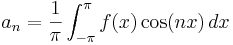
and
are called the Fourier coefficients of ƒ. The infinite sum
![\frac{a_0}{2} +\sum_{n=1}^{\infty}[a_n \cos(nx) + b_n \sin(nx)]](/2009-wikipedia_en_wp1-0.7_2009-05/I/7fb5b800bcb20fb81477f7d829c9fe90.png)
is the Fourier series for ƒ on the interval [−π, π].
The Fourier series does not always converge, and even when it does the value of the series may differ from the value of the function. It is one of the main questions in Harmonic analysis to decide when it converges and when it is equal to the original function. If a function is square-integrable on the interval [−π, π], then the Fourier series converges to the function at almost every point. In engineering applications, the Fourier series is generally presumed to converge everywhere except at discontinuities, since the functions encountered in engineering are more well behaved than the ones that mathematicians can provide as counter-examples to this presumption. In particular, the Fourier series converges absolutely and uniformly to ƒ(x) whenever the derivative of ƒ(x) (which may not exist everywhere) is square integrable.[2] See Convergence of Fourier series.
It is possible to define Fourier coefficients for more general functions or distributions, in such cases convergence in norm or weak convergence is usually of interest.
Example: a simple Fourier series

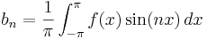
We now use the formulae above to give a Fourier series expansion of a very simple function. Consider a sawtooth function (as depicted in the figure):


In this case, the Fourier coefficients are given by
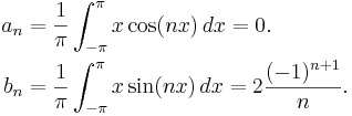
And therefore:
|
|
|
( |
|
|
![\begin{align}
f(x) &= \frac{a_0}{2} + \sum_{n=1}^{\infty}\left[a_n\cos\left(nx\right)+b_n\sin\left(nx\right)\right] \\
&=2\sum_{n=1}^{\infty}\frac{(-1)^{n+1}}{n} \sin(nx), \quad \mathrm{for} \quad -\infty < x < \infty .
\end{align}](/2009-wikipedia_en_wp1-0.7_2009-05/I/d75778cf6426e2c98517c9e29c959646.png)

One notices that the Fourier series expansion of our function looks much less simple than the formula ƒ(x) = x, and so it is not immediately apparent why one would need this Fourier series. While there are many applications, we cite Fourier's motivation of solving the heat equation. For example, consider a metal plate in the shape of a square whose side measures π meters, with coordinates (x, y) ∈ [0, π] × [0, π]. If there is no heat source within the plate, and if three of the four sides are held at 0 degrees Celsius, while the fourth side, given by y = π, is maintained at the temperature gradient T(x, π) = x degrees Celsius, for x in (0, π), then one can show that the stationary heat distribution (or the heat distribution after a long period of time has elapsed) is given by
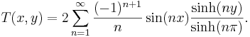
Here, sinh is the hyperbolic sine function. This solution of the heat equation is obtained by multiplying each term of Eq.1 by sinh(ny)/sinh(nπ). While our example function f(x) seems to have a needlessly complicated Fourier series, the heat distribution T(x, y) is nontrivial. The function T cannot be written as a closed-form expression. This method of solving the heat problem was only made possible by Fourier's work.
Another application of this Fourier series is to solve the Basel problem by using Parseval's theorem. The example generalizes and one may compute ζ(2n), for any positive integer n.
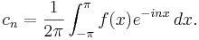
The modern version using complex exponentials
We can use Euler's formula,
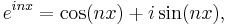
where  is the imaginary unit, to give a more concise formula:
The Fourier coefficients are then given by:
The Fourier coefficients  are related via
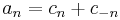 for
for 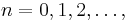
and
 for
for 
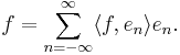
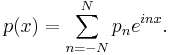
The notation cn is inadequate for discussing the Fourier coefficients of several different functions. Therefore it is customarily replaced by a modified form of ƒ (in this case), such as F or  and functional notation often replaces subscripting. Thus:
![\begin{align}
f(x) &= \sum_{n=-\infty}^{\infty} \hat{f}(n)\cdot e^{inx} \\
&= \sum_{n=-\infty}^{\infty} F[n]\cdot e^{inx} \quad \mbox{(engineering)}.
\end{align}](/2009-wikipedia_en_wp1-0.7_2009-05/I/404d6e7a78b18521aa2d32f6c70240fd.png)
In engineering, particularly when variable x represents time, the coefficient sequence is called a frequency domain representation. Square brackets are often used to emphasize that the domain of this function is a discrete set of frequencies.
Fourier series on a general interval [a, b]
The following formula, with appropriate complex-valued coefficients G[n], is a periodic function with period τ on all of R:
![g(x)=\sum_{n=-\infty}^\infty G[n]\cdot e^{i 2\pi \frac{n}{\tau} x}\ .](/2009-wikipedia_en_wp1-0.7_2009-05/I/a175791c6d1eb7b82bb2c32c5906b4fb.png)
If a function is square-integrable in the interval [a, a + τ], it can be represented in that interval by the formula above. If g(x) is integrable, then the Fourier coefficients are given by:
![G[n] = \frac{1}{\tau}\int_a^{a+\tau} g(x)\cdot e^{-i 2\pi \frac{n}{\tau} x}\, dx.](/2009-wikipedia_en_wp1-0.7_2009-05/I/61a37ec6e60114cc4c1c034156ad94b8.png)
Note that if the function to be represented is also τ-periodic, then a is an arbitrary choice. Two popular choices are a = 0, and a = −τ/2.
Another commonly used frequency domain representation uses the Fourier series coefficients to modulate a Dirac comb:
![G(f) \ \stackrel{\mathrm{def}}{=} \ \sum_{n=-\infty}^{\infty} G[n]\cdot \delta \left(f-\frac{n}{\tau}\right)](/2009-wikipedia_en_wp1-0.7_2009-05/I/ec5b15aee84257a616ce867656034901.png)
where variable ƒ represents a continuous frequency domain. When variable x has units of seconds, ƒ has units of hertz. The "teeth" of the comb are spaced at multiples (i.e. harmonics) of 1/τ, which is called the fundamental frequency. The original g(x) can be recovered from this representation by an inverse Fourier transform:
![\begin{align}
\mathcal{F}^{-1}\{G(f)\} &=
\mathcal{F}^{-1}\left\{ \sum_{n=-\infty}^{\infty} G[n]\cdot \delta \left(f-\frac{n}{\tau}\right)\right\}\\
&= \sum_{n=-\infty}^{\infty} G[n]\cdot \underbrace{\mathcal{F}^{-1}\left\{\delta\left(f-\frac{n}{\tau}\right)\right\}}_{e^{i2\pi \frac{n}{\tau} x}\cdot \underbrace{\mathcal{F}^{-1}\{\delta (f)\}}_{1}}\\
&= \sum_{n=-\infty}^{\infty} G[n]\cdot e^{i2\pi \frac{n}{\tau} x} \quad = \ \ g(x).
\end{align}](/2009-wikipedia_en_wp1-0.7_2009-05/I/9cad761f48f4b08af25320026114f295.png)
The function  is therefore commonly referred to as a Fourier transform, even though the Fourier integral of a periodic function is not convergent.[3]
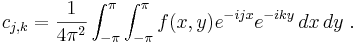
Fourier series on a square
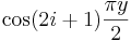
We can also define the Fourier series for functions of two variables x and y in the square [−π, π]×[−π, π]:
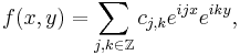
Aside from being useful for solving partial differential equations such as the heat equation, one notable application of Fourier series on the square is in image compression. In particular, the jpeg image compression standard uses the two-dimensional discrete cosine transform, which is a Fourier transform using the cosine basis functions.
Hilbert space interpretation
In the language of Hilbert spaces, the set of functions  is an orthonormal basis for the space
 ![L^2([-\pi,\pi])](/2009-wikipedia_en_wp1-0.7_2009-05/I/3d8f180a154f929df8f6489100bd256b.png) of square-integrable functions of
of square-integrable functions of ![[-\pi,\pi]](/2009-wikipedia_en_wp1-0.7_2009-05/I/911bebeafbf3d4845e122edfc4f667f8.png) . This space is actually a Hilbert space with an inner product given by:
. This space is actually a Hilbert space with an inner product given by:

The basic Fourier series result for Hilbert spaces can be written as
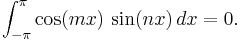
This corresponds exactly to the complex exponential formulation given above. The version with sines and cosines is also justified with the Hilbert space interpretation. Clearly, the sines and cosines form an orthonormal set:

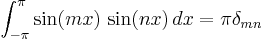
(where  is the Kronecker delta), and
The density of their span is a consequence of the Stone-Weierstrass theorem.
Properties
We say that  if
if  is a function of
  which is
  times differentiable, its kth derivative is continuous, and is
  -periodic.
- If f is a -periodic odd function, then
 for all
  .
.
- If f is a -periodic even function, then
 for all .
- If f is integrable,
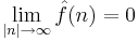 ,
,  and
and  This result is known as the Riemann-Lebesgue Lemma.
- If
 , then the Fourier coefficients
  of the derivative
  can be expressed in terms of the Fourier coefficients
  of the function
  , via the formula
  .
.
- If , then
 . In particular, since
  tends to zero, we have that
  tends to zero, which means that the Fourier coefficients converge to zero faster than the kth power of n.
- Parseval's theorem. If
![f \in L^2([-\pi,\pi])](/2009-wikipedia_en_wp1-0.7_2009-05/I/e6ac7960b924290b4dfe0e149c47a691.png) , then
, then  .
.
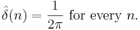
- Plancherel's theorem. If
 are coefficients and
 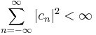 then there is a unique function such that
  for every .
- The Convolution theorem states that if f and g are in , then
 , where
  denotes the -periodic convolution of f and g.
General case
There are many possible avenues for generalizing Fourier series. The study of Fourier series and its generalizations is called Harmonic analysis.
Generalized functions
One can extend the notion of Fourier coefficients to functions which are not square-integrable, and even to objects which are not functions. This is very useful in engineering and applications because we often need to take the Fourier series of a periodic repetition of a Dirac delta function. The Dirac delta δ is not actually a function; still, it has a Fourier transform and its periodic repetition has a Fourier series:
This generalization to distributions enlarges the domain of definition of the Fourier transform from L2([−π, π]) to a superset of L2. The Fourier series converges weakly.
Compact groups
One of the interesting properties of the Fourier transform which we have mentioned, is that it carries convolutions to pointwise products. If that is the property which we seek to preserve, one can produce Fourier series on any compact group. Typical examples include those classical groups that are compact. This generalizes the Fourier transform to all spaces of the form L2(G), where G is a compact group, in such a way that the Fourier transform carries convolutions to pointwise products. The Fourier series exists and converges in similar ways to the [−π, π] case.
Riemannian manifolds
If the domain is not a group, then there is no intrinsically defined convolution. However, if  is a compact Riemannian manifold, it has a Laplace-Beltrami operator. The Laplace-Beltrami operator is the differential operator that corresponds to Laplace operator for the Riemannian manifold . Then, by analogy, one can consider heat equations on . Since Fourier arrived at his basis by attempting to solve the heat equation, the natural generalization is to use the eigensolutions of the Laplace-Beltrami operator as a basis. This generalizes Fourier series to spaces of the type
  , where is a Riemannian manifold. The Fourier series converges in ways similar to the case. A typical example is to take X to be the sphere with the usual metric, in which case the Fourier basis consists of spherical harmonics.
Locally compact Abelian groups
The generalization to compact groups discussed above does not generalize to noncompact, nonabelian groups. However, there is a straightfoward generalization to Locally Compact Abelian (LCA) groups.
This generalizes the Fourier transform to  or
or  , where G is an LCA group. If
  is compact, one also obtains a Fourier series, which converges similarly to the case, but if is noncompact, one obtains instead a Fourier integral. This generalization yields the usual Fourier transform when the underlying locally compact Abelian group is .
Approximation and convergence of Fourier series
An important question for the theory as well as applications is that of convergence. In particular, it is often necessary in applications to replace the infinite series  by a finite one,
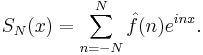
This is called a partial sum. We would like to know, in which sense does SN(x) converge to f(x) as N tends to infinity.
Least squares property
We say that p is a trigonometric polynomial of degree N when it is of the form
Note that  is a trigonometric polynomial of degree N. Parseval's theorem implies that
Theorem. is the unique best trigonometric polynomial of degree  approximating
  , in the sense that, for any trigonometric polynomial
  of degree , we have
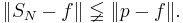
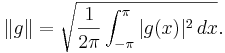
Here, the Hilbert space norm is
Convergence
Because of the least squares property, and because of the completeness of the Fourier basis, we obtain an elementary convergence result.
Theorem. If , then the Fourier series converges in , that is,  converges to 0 as goes to infinity.
We have already mentioned that if f is twice continuously differentiable, then  converges to zero as n goes to infinity. This immediately gives a second convergence result.
Theorem. If  , then
 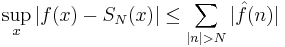 converges to zero, i.e.,
  converges to uniformly.
In particular, converges to f pointwise.
Many further cases are discussed in the main article, Convergence of Fourier series, ranging from the moderately simple result that the series converges at x if f is differentiable at x, to Lennart Carleson's much more sophisticated result that the Fourier series of an  function actually converges almost everywhere.
Divergence
Since Fourier series have such good convergence properties, many are often surprised by some of the negative results. For example, the Fourier series of a continuous T-periodic function need not converge pointwise.
In 1922, Andrey Kolmogorov published an article entitled "Une série de Fourier-Lebesgue divergente presque partout" in which he gave an example of a Lebesgue-integrable function whose Fourier series diverges almost everywhere. He later constructed an example of an integrable function whose Fourier series diverges everywhere (Katznelson 1976).
See also
- Gibbs phenomenon
- Laurent series — the substitution
 transforms a Fourier series into a Laurent series, or conversely. This is used in the q-series expansion of the j-invariant.
 - Sturm-Liouville theory
Notes
- ↑ Gallica - Fourier, Jean-Baptiste-Joseph (1768-1830). Oeuvres de Fourier. 1888
- ↑ Georgi P. Tolstov (1976). Fourier Series. Courier-Dover. ISBN 0486633179. http://books.google.com/books?id=XqqNDQeLfAkC&pg=PA82&dq=fourier-series+converges+continuous-function&ei=L0rJSMvANIPsswOs-pzXDA&sig=ACfU3U3teR3Wwlu7HYq_qHV4QZqj6sYP5A.
- ↑ Since the integral defining the Fourier transform of a periodic function is not convergent, it is necessary to view the periodic function and its transform as distributions. In this sense
 is a Dirac delta function, which is an example of a distribution.
References
- William E. Boyce and Richard C. DiPrima, Elementary Differential Equations and Boundary Value Problems, Eighth edition. John Wiley & Sons, Inc., New Jersey, 2005. ISBN 0-471-43338-1
- Joseph Fourier, translated by Alexander Freeman (published 1822, translated 1878, re-released 2003). The Analytical Theory of Heat. Dover Publications. ISBN 0-486-49531-0. 2003 unabridged republication of the 1878 English translation by Alexander Freeman of Fourier's work Théorie Analytique de la Chaleur, originally published in 1822.
- Katznelson, Yitzhak (1976), An introduction to harmonic analysis (Second corrected ed.), New York: Dover Publications, Inc, ISBN 0-486-63331-4
- Felix Klein, Development of mathematics in the 19th century. Mathsci Press Brookline, Mass, 1979. Translated by M. Ackerman from Vorlesungen über die Entwicklung der Mathematik im 19 Jahrhundert, Springer, Berlin, 1928.
- Walter Rudin, Principles of mathematical analysis, Third edition. McGraw-Hill, Inc., New York, 1976. ISBN 0-07-054235-X
External links
- Phasor Phactory Allows custom control of the harmonic amplitudes for arbitrary terms
- Java applet shows Fourier series expansion of an arbitrary function
- Example problems - Examples of computing Fourier Series
- Fourier series explanation - A simple, non-mathematical approach
- Eric W. Weisstein, Fourier Series at MathWorld.
- Fourier Series Module by John H. Mathews
- Joseph Fourier - A site on Fourier's life which was used for the historical section of this article
- In the bottom of this interactive lecture, there is a Java animation showing how the Fourier series is affected when the term of rank n+1 is added to the n Fourier series terms.
This article incorporates material from example of Fourier series on PlanetMath, which is licensed under the GFDL.