Differential form

In the mathematical fields of differential geometry and tensor calculus, differential forms are an approach to multivariable calculus which is independent of coordinates. A differential form of degree k, or (differential) k-form, on a smooth manifold M is a smooth section of the kth exterior power of the cotangent bundle of M. The set of all k-forms on M is a vector space commonly denoted Ω^k(M).

A differential 0-form is by definition a smooth function on M. A differential 1-form is an object dual to a vector field on M.

Differential forms can be multiplied together using an operation called the wedge product. There is also a differential operator on differential forms called the exterior derivative. The wedge product of a k-form and an l-form is a (k+l)-form, and the exterior derivative of a k-form is a (k+1)-form. In particular, the exterior derivative of a 0-form (which is a function on M) is its differential (which is a 1-form on M).

The modern notion of differential forms was pioneered by Élie Cartan, and has many applications, especially in geometry, topology and physics.

1 Concept
2 Intrinsic definitions
3 Operations
4 Exterior differential complex
5 Pullback
6 Integration
7 Applications in physics
8 Applications in geometric measure theory
9 See also
10 References
11 External links

Concept

Differential forms provide an approach to multivariable calculus which is independent of coordinates.

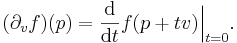
Let U be an open set in Rⁿ. A differential 0-form ("zero form") is defined to be a smooth function f on U. If v is any vector in Rⁿ, then f has a directional derivative ∂_v f, which is another function on U whose value at a point p∈U is the rate of change (at p) of f in the v direction:

$(\partial_v f)(p) = \frac{\mathrm d}{ \mathrm d t} f(p+tv)\Big|_{t=0}.$

(This notion can be extended to the case that v is a vector field on U by evaluating v at the point p in the definition.)

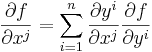
In particular, if v=e_j is the jth coordinate vector then ∂_vf is the partial derivative of f with respect to the jth coordinate function, i.e., ∂f / ∂x^j, where x¹, x²,... xⁿ are the coordinate functions on U. By their very definition, partial derivatives depend upon the choice of coordinates: if new coordinates y¹ , y²,... yⁿ are introduced, then

$\frac{\partial f}{\partial x^j} = \sum_{i=1}^n\frac{\partial y^i}{\partial x^j}\frac{\partial f}{\partial y^i}$

The first idea leading to differential forms is the observation that ∂_v f (p) is a linear function of v:

$(\partial_{v+w} f)(p) = (\partial_v f)(p) + (\partial_w f)(p)$

$(\partial_{c v} f)(p) = c (\partial_v f)(p)$

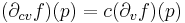
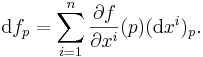
for any vectors v, w and any real number c. This linear map from Rⁿ to R is denoted df_p and called the derivative of f at p. Thus df_p(v) = ∂_v f (p). The object df can be viewed as a function on U, whose value at p is not a real number, but the linear map df_p. This is an example of a differential 1-form.

Since any vector v is a linear combination ∑ v^je_j of its components, df is uniquely determined by df_p(e_j) for each j and each p∈U, which are just the partial derivatives of f on U. Thus df provides a way of encoding the partial derivatives of f. It can be decoded by noticing that the coordinates x¹, x²,... xⁿ are themselves functions on U, and so define differential 1-forms dx¹, dx²,... dxⁿ. Since ∂xⁱ / ∂x^j = δ_ij, the Kronecker delta function, it follows that

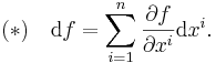
$(*)\quad \mathrm d f = \sum_{i=1}^n \frac{\partial f}{\partial x^i} \mathrm{d} x^i.$

The meaning of this expression is given by evaluating both sides at an arbitrary point p: on the right hand side, the sum is defined "pointwise", so that

$\mathrm d f_p = \sum_{i=1}^n \frac{\partial f}{\partial x^i}(p) (\mathrm{d} x^i)_p.$

Applying both sides to e_j, the result on each side is the jth partial derivative of f at p. Since p and j were arbitrary, this proves the formula (*).

More generally, for any smooth functions g_i and h_i on U, we define the differential 1-form α = ∑_i g_i dh_i pointwise by

$\alpha_p = \sum_i g_i(p) (\mathrm d h_i)_p\,\!$

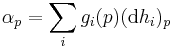
for each p∈U. Any differential 1-form arises this way, and by using (*) it follows that any differential 1-form α on U may be expressed in coordinates as

$\alpha = \sum_{i=1}^n f_i\, \mathrm{d} x^i$

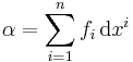
for some smooth functions f_i on U.

The second idea leading to differential forms arises from the following question: given a differential 1-form α on U, when does there exist a function f on U such that α = df? The above expansion reduces this question to the search for a function f whose partial derivatives ∂f / ∂xⁱ are equal to n given functions f_i. For n>1, such a function does not always exist: any smooth function f satisfies

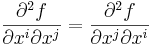
$\frac{\partial^2 f}{\partial x^i\partial x^j} = \frac{\partial^2 f}{\partial x^j\partial x^i}$

so it will be impossible to find such an f unless

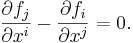
$\frac{\partial f_j}{\partial x^i} - \frac{\partial f_i}{\partial x^j}=0.$

for all i and j.

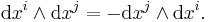
The skew-symmetry of the left hand side in i and j suggests introducing an antisymmetric product $\wedge$ on differential 1-forms, the wedge product, so that these equations can be combined into a single condition

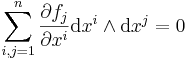
$\sum_{i,j=1}^n \frac{\partial f_j}{\partial x^i} {\mathrm d}x^i \wedge {\mathrm d}x^j = 0$

where

${\mathrm d}x^i \wedge {\mathrm d}x^j = - {\mathrm d}x^j \wedge {\mathrm d}x^i.$

This is an example of a differential 2-form: the exterior derivative dα of α= ∑_j=1ⁿ f_j dx^j is given by

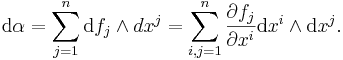
$\mathrm d\alpha = \sum_{j=1}^n \mathrm d f_j \wedge dx^j = \sum_{i,j=1}^n \frac{\partial f_j}{\partial x^i} {\mathrm d}x^i \wedge {\mathrm d}x^j.$

To summarize: dα = 0 is a necessary condition for the existence of a function f with α=df.

Differential 0-forms, 1-forms, and 2-forms are special cases of differential forms. For each k, there is a space of differential k-forms, which can be expressed in terms of the coordinates as

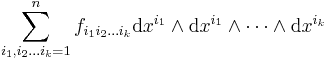
$\sum_{i_1,i_2\ldots i_k=1}^n f_{i_1i_2\ldots i_k} \mathrm d x^{i_1} \wedge\mathrm d x^{i_1} \wedge\cdots \wedge \mathrm d x^{i_k}$

for a collection of functions f_{i₁i₂...i_k}.

Differential forms can be multiplied together using the wedge product, and for any differential k-form α, there is a differential (k+1)-form dα called the exterior derivative of α.

Differential forms, the wedge product and the exterior derivative are independent of a choice of coordinates. Consequently they may be defined on any smooth manifold M. One way to do this is cover M with coordinate charts and define a differential k-form on M to be a a family of differential k-forms on each chart which agree on the overlaps. However, there are more intrinsic definitions which make the independence of coordinates manifest.

Intrinsic definitions

Let M be a smooth manifold. A differential form of degree k is a smooth section of the kth exterior power of the cotangent bundle of M. At any point p∈M, a k-form β defines an alternating multilinear map

$\beta_p\colon T_p M\times \cdots \times T_p M \to \mathbb{R}$

(with k factors of T_pM in the product), where T_pM is the tangent space to M at p. Equivalently, β is a totally antisymmetric covariant tensor field of rank k.

The set of all differential k-forms on a manifold M is a vector space, often denoted Ω^k(M).

For example, a differential 1-form α assigns to each point p∈M a linear functional α_p on T_pM. In the presence of an inner product on T_pM (induced by a Riemannian metric on M), α_p may be represented as the inner product with a tangent vector X_p. Differential 1-forms are sometimes called covariant vector fields, covector fields, or "dual vector fields", particular within physics.

Operations

There are several operations on differential forms: wedge product, exterior derivative, interior product and Lie derivative.

The wedge product of a k-form α and an l-form β is a (k+l)-form denoted αΛβ. For example, if k=l=1, then αΛβ is the 2-form whose value at a point p is the alternating bilinear form defined by

$(\alpha\wedge\beta)_p(v,w)=\alpha_p(v)\beta_p(w) - \alpha_p(w)\beta_p(v)$

for v, w ∈ T_pM. (In an alternative convention, the right hand side is divided by two in this formula.)

The wedge product is bilinear: for instance, if α, β, and γ are any differential forms, then

$\alpha \wedge (\beta + \gamma) = \alpha \wedge \beta + \alpha \wedge \gamma.$

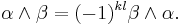
It is skew commutative (also known as graded commutative), meaning that it satisfies a variant of anticommutativity that depends on the degrees of the forms: if α is a k-form and β is an l-form, then

$\alpha \wedge \beta = (-1)^{kl} \beta \wedge \alpha.$

Exterior differential complex

One important property of the exterior derivative is that d² = 0. This means that the exterior derivative defines a cochain complex:

$0 \to\Omega^0(M)\ \stackrel{\mathrm d}{\to}\ \Omega^1(M)\ \stackrel{\mathrm d}{\to}\ \Omega^2(M)\ \stackrel{\mathrm d}{\to}\ \Omega^3(M) \to \cdots$

where i is the inclusion of constant functions. By the Poincaré lemma, this complex is locally exact except at Ω⁰(M). Its cohomology is the de Rham cohomology of M.

On a Riemannian manifold, additional operations, such as the Hodge star operator and codifferential can be defined.

Pullback

See also: Pullback (differential geometry)

One of the main reasons the cotangent bundle rather than the tangent bundle is used in the construction of the exterior complex is that differential forms are capable of being pulled back by smooth maps, while vector fields cannot be pushed forward by smooth maps unless the map is, say, a diffeomorphism. The existence of pullback homomorphisms in de Rham cohomology depends on the pullback of differential forms.

Differential forms can be moved from one manifold to another using a smooth map. If f : M → N is smooth and ω is a smooth k-form on N, then there is a differential form f^*ω on M, called the pullback of ω, which captures the behavior of ω as seen relative to f.

To define the pullback, recall that the differential of f is a map f_* : TM → TN. Fix a differential k-form ω on N. For a point p of M and tangent vectors v₁, ..., v_k to M at p, the pullback of ω is defined by the formula

$(f^*\omega)_p(v_1, \ldots, v_k) = \omega_{f(p)}(f_*v_1, \ldots, f_*v_k).$

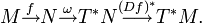
More abstractly, if ω is viewed as a section of the cotangent bundle T^*N of N, then f^*ω is the section of T^*M defined as the composite map

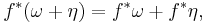
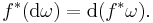
$M \stackrel{f}{\to} N \stackrel{\omega}{\to} T^*N \stackrel{(Df)^*}{\longrightarrow} T^*M.$

Pullback respects all of the basic operations on forms:

$f^*(\omega + \eta) = f^*\omega + f^*\eta,$

$f^*(\omega\wedge\eta) = f^*\omega\wedge f^*\eta,$

$f^*(\mathrm{d}\omega) = \mathrm{d}(f^*\omega).$

The pullback of a form can also be written in coordinates. Assume that x₁, ..., x_m are coordinates on M, that y₁, ..., y_n are coordinates on N, and that these coordinate systems are related by the formulas y_i = f_i(x₁, ..., x_m) for all i. Then, locally on N, ω can be written as

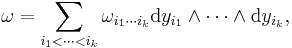
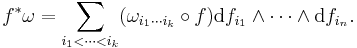
$\omega = \sum_{i_1 < \cdots < i_k} \omega_{i_1\cdots i_k}\mathrm{d}y_{i_1} \wedge \cdots \wedge \mathrm{d}y_{i_k},$

where, for each choice of i₁, ..., i_k, $\omega_{i_1\cdots i_k}$ is a real-valued function of y₁, ..., y_n. Using the linearity of pullback and its compatibility with wedge product, the pullback of ω has the formula

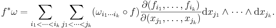
$f^*\omega = \sum_{i_1 < \cdots < i_k} (\omega_{i_1\cdots i_k}\circ f)\mathrm{d}f_{i_1}\wedge\cdots\wedge\mathrm{d}f_{i_n}.$

Each exterior derivative df_i can be expanded in terms of dx₁, ..., dx_m. The resulting k-form can be written using Jacobian matrices:

$f^*\omega = \sum_{i_1 < \cdots < i_k} \sum_{j_1 < \cdots < j_k} (\omega_{i_1\cdots i_k}\circ f)\frac{\partial(f_{i_1}, \ldots, f_{i_k})}{\partial(x_{j_1}, \ldots, x_{j_k})}\mathrm{d}x_{j_1} \wedge \cdots \wedge\mathrm{d}x_{j_k}.$

Integration

Differential forms of degree k are integrated over k dimensional chains. If k = 0, this is just evaluation of functions at points. Other values of k = 1, 2, 3, ... correspond to line integrals, surface integrals, volume integrals etc.

Let

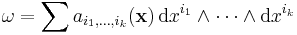
$\omega=\sum a_{i_1,\dots,i_k}({\mathbf x})\,{\mathrm d}x^{i_1} \wedge \cdots \wedge {\mathrm d}x^{i_k}$

be a differential form and S a differentiable k-manifold over which we wish to integrate, where S has the parameterization

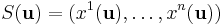
$S({\mathbf u})=(x^1({\mathbf u}),\dots,x^n({\mathbf u}))$

for u in the parameter domain D. Then [Rudin, 1976] defines the integral of the differential form over S as

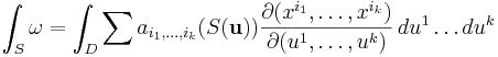
$\int_S \omega =\int_D \sum a_{i_1,\dots,i_k}(S({\mathbf u})) \frac{\partial(x^{i_1},\dots,x^{i_k})}{\partial(u^{1},\dots,u^{k})}\,du^1\ldots du^k$

where

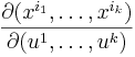
$\frac{\partial(x^{i_1},\dots,x^{i_k})}{\partial(u^{1},\dots,u^{k})}$

is the determinant of the Jacobian. The Jacobian exists because S is differentiable.

The fundamental relationship between the exterior derivative and integration is given by the general Stokes' theorem: If $\omega$ is an n−1-form with compact support on M and ∂M denotes the boundary of M with its induced orientation, then

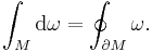
$\int_M \mathrm {d}\omega = \oint_{\partial M} \omega.\!\,$

This theorem also underlies the duality between de Rham cohomology and the homology of chains.

Applications in physics

Differential forms arise in some important physical contexts. For example, in Maxwell's theory of electromagnetism, the Faraday 2-form or electromagnetic field strength is

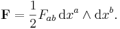
$\textbf{F} = \frac{1}{2}F_{ab}\, {\mathrm d}x^a \wedge {\mathrm d}x^b.$

Note that this form is a special case of the curvature form on the U(1) principal fiber bundle on which both electromagnetism and general gauge theories may be described. The current 3-form is

$\textbf{J} = J^a \epsilon_{abcd}\, {\mathrm d}x^b \wedge {\mathrm d}x^c \wedge {\mathrm d}x^d.$

Using these definitions, Maxwell's equations can be written very compactly in geometrized units as

$\mathrm{d}\, {\textbf{F}} = \textbf{0}$

$\mathrm{d}\, {*\textbf{F}} = \textbf{J}$

where $*$ denotes the Hodge star operator. Similar considerations describe the geometry of gauge theories in general.

The 2-form $* \mathbf{F}$ is also called Maxwell 2-form.

Applications in geometric measure theory

Numerous minimality results for complex analytic manifolds are based on the Wirtinger inequality for 2-forms. A succinct proof may be found in Herbert Federer's classic text Geometric Measure Theory. The Wirtinger inequality is also a key ingredient in Gromov's inequality for complex projective space in systolic geometry.

References

Bachman, David (2006), A Geometric Approach to Differential Forms, Birkhauser, ISBN 978-0-8176-4499-4
Flanders, Harley (1989), Differential forms with applications to the physical sciences, Mineola, NY: Dover Publications, ISBN 0-486-66169-5
Fleming, Wendell H. (1965), "Chapter 6: Exterior algebra and differential calculus", Functions of Several Variables, Addison-Wesley, pp. 205–238 . This textbook in multivariate calculus introduces the exterior algebra of differential forms at the college calculus level
Morita, Shigeyuki (2001), Geometry of Differential Forms, AMS, ISBN 0-8218-1045-6
Rudin, Walter (1976), Principles of Mathematical Analysis, New York: McGraw-Hill, ISBN 0-07-054235-X
Spivak, Michael (1965), Calculus on Manifolds, Menlo Park, CA: W. A. Benjamin, ISBN 0-8053-9021-9
Zorich, Vladimir A. (2004), Mathematical Analysis II, Springer, ISBN 3-540-40633-6

External links

Eric W. Weisstein, Differential form at MathWorld.
Sjamaar, Reyer (2006), Manifolds and differential forms lecture notes, http://www.math.cornell.edu/~sjamaar/classes/321/notes.html , a course taught at Cornell University.