Curvature
In mathematics, curvature refers to any of a number of loosely related concepts in different areas of geometry. Intuitively, curvature is the amount by which a geometric object deviates from being flat, or straight in the case of a line, but this is defined in different ways depending on the context. There is a key distinction between extrinsic curvature, which is defined for objects embedded in another space (usually a Euclidean space) in a way that relates to the radius of curvature of circles that touch the object, and intrinsic curvature, which is defined at each point in a differential manifold. This article deals primarily with the first concept.
The primordial example of extrinsic curvature is that of a circle, which has curvature equal to the inverse of its radius everywhere. Smaller circles bend more sharply, and hence have higher curvature. The curvature of a smooth curve is defined as the curvature of its osculating circle at each point.
In a plane, this is a scalar quantity, but in three or more dimensions it is described by a curvature vector that takes into account the direction of the bend as well as its sharpness. The curvature of more complex objects (such as surfaces or even curved n-dimensional spaces) is described by more complex objects from linear algebra, such as the general Riemann curvature tensor.
The remainder of this article discusses, from a mathematical perspective, some geometric examples of curvature: the curvature of a curve embedded in a plane and the curvature of a surface in Euclidean space. See the links below for further reading.
Contents |
One dimension in two dimensions: Curvature of plane curves
For a plane curve C, the mathematical definition of curvature uses a parametric representation of C with respect to the arc length parametrization. It can be computed given any regular parametrization by a more complicated formula given below. Let γ(s) be a regular parametric curve, where s is the arc length, or natural parameter. This determines the unit tangent vector T, the unit normal vector N, the curvature κ(s), the oriented or signed curvature k(s), and the radius of curvature at each point:

The curvature of a straight line is identically zero. The curvature of a circle of radius R is constant, i.e. it does not depend on the point and is equal to the reciprocal of the radius:

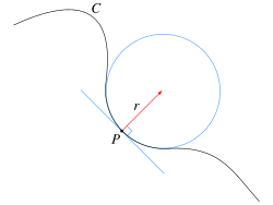
Thus for a circle, the radius of curvature is simply its radius. Straight lines and circles are the only plane curves whose curvature is constant. Given any curve C and a point P on it where the curvature is non-zero, there is a unique circle which most closely approximates the curve near P, the osculating circle at P. The radius of the osculating circle is the radius of curvature of C at this point.
The meaning of curvature
Suppose that a particle moves on the plane with unit speed. Then the trajectory of the particle will trace out a curve C in the plane. Moreover, taking the time as the parameter, this provides a natural parametrization for C. The instanteneous direction of motion is given by the unit tangent vector T and the curvature measures how fast this vector rotates. If a curve keeps close to the same direction, the unit tangent vector changes very little and the curvature is small; where the curve undergoes a tight turn, the curvature is large.
The magnitude of curvature at points on physical curves can be measured in diopters (also spelled dioptre) — this is the convention in optics. A diopter has the dimension 
Signed curvature
The sign of the signed curvature k indicates the direction in which the unit tangent vector rotates as a function of the parameter along the curve. If the unit tangent rotates counterclockwise, then k > 0. If it rotates clockwise, then k < 0.
The signed curvature depends on the particular parametrization chosen for a curve. For example the unit circle can be parametrised by  (counterclockwise, with k > 0), or by
  (clockwise, with k < 0). More precisely, the signed curvature depends only on the choice of orientation of an immersed curve. Every immersed curve in the plane admits two possible orientations.
Local expressions
- See also: Centripetal force#Alternative approach
For a plane curve given parametrically as  , the curvature is
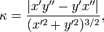
and the signed curvature k is
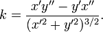
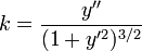
For the less general case of a plane curve given explicitly as  the curvature is

Slightly abusing notation, the signed curvature may also be written in this way as
with the understanding that the curve is traversed in the direction of increasing x.
This quantity is common in physics and engineering; for example, in the equations of bending in beams, the 1D vibration of a tense string, approximations to the fluid flow around surfaces (in aeronautics), and the free surface boundary conditions in ocean waves. In such applications, the assumption is almost always made that the slope is small compared with unity, so that the approximation:

may be used. This approximation yields a straightforward linear equation describing the phenomenon, which would otherwise remain intractable.
If a curve is defined in polar coordinates as  , then its curvature is

where here the prime refers to differentiation with respect to  .
.
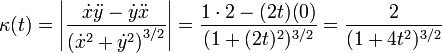
Example
Consider the parabola  . We can parametrize the curve simply as
  ,
,

Substituting
One dimension in three dimensions: Curvature of space curves
- See Frenet-Serret formulas for a fuller treatment of curvature and the related concept of torsion.
For a parametrically defined space curve as  , its curvature is:
![F[x,y,z]=\frac{\sqrt{(z''y'-y''z')^2+(x''z'-z''x')^2+(y''x'-x''y')^2}}{(x'^2+y'^2+z'^2)^{3/2}}](/2009-wikipedia_en_wp1-0.7_2009-05/I/4d3cc6deba79103effa6aab760011598.png)
Given a function r(t) with values in R3, the curvature at a given value of  is
is

where  and
and  correspond to the first and second derivatives of r(t), respectively. (Note that this formula is the vector notation of F[x,y,z] above.)
Curves on surfaces
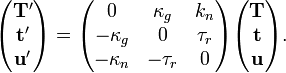
When a one dimensional curve lies on a two dimensional surface embedded in three dimensions R3, further measures of curvature are available, which take the surface's unit-normal vector, u into account. These are the normal curvature, geodesic curvature and geodesic torsion. Any non-singular curve on a smooth surface will have its tangent vector T lying in the tangent plane of the surface orthogonal to the normal vector. The normal curvature, kn, is the curvature of the curve projected onto the plane containing the curves tangent T and the surface normal u; the geodesic curvature, kg, is the curvature of the curve projected onto the surfaces tangent plane; and the geodesic torsion (or relative torsion), τr, measures the rate of change of the surface normal around the curves tangent.
Let the curve be a unit speed curve and let t = u × T so that T, u, t form an orthonormal basis: the Darboux frame. The quantities k, g and τ are related by:
Principal curvature

All curves with the same tangent vector will have the same normal curvature, which is the same as the curvature of the curve obtained by intersecting the surface with the plane containing T and u. Taking all possible tangent vectors then the maximum and minimum values of the normal curvature at a point are called the principal curvatures, k1 and k2, and the directions of the corresponding tangent vectors are called principal directions.
Two dimensions: Curvature of surfaces
Gaussian curvature
In contrast to curves, which do not have intrinsic curvature, but do have extrinsic curvature (they only have a curvature given an embedding), surfaces have intrinsic curvature, independent of an embedding.
Here we adopt the convention that a curvature is taken to be positive if the curve turns in the same direction as the surface's chosen normal, otherwise negative.
The Gaussian curvature, named after Carl Friedrich Gauss, is equal to the product of the principal curvatures, k1k2. It has the dimension of 1/length2 and is positive for spheres, negative for one-sheet hyperboloids and zero for planes. It determines whether a surface is locally convex (when it is positive) or locally saddle (when it is negative).
The above definition of Gaussian curvature is extrinsic in that it uses the surface's embedding in R3, normal vectors, external planes etc. Gaussian curvature is however in fact an intrinsic property of the surface, meaning it does not depend on the particular embedding of the surface; intuitively, this means that ants living on the surface could determine the Gaussian curvature. Formally, Gaussian curvature only depends on the Riemannian metric of the surface. This is Gauss' celebrated Theorema Egregium, which he found while concerned with geographic surveys and mapmaking.
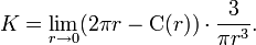
An intrinsic definition of the Gaussian curvature at a point P is the following: imagine an ant which is tied to P with a short thread of length r. She runs around P while the thread is completely stretched and measures the length C(r) of one complete trip around P. If the surface were flat, she would find C(r) = 2πr. On curved surfaces, the formula for C(r) will be different, and the Gaussian curvature K at the point P can be computed by the Bertrand–Diquet–Puiseux theorem as
The integral of the Gaussian curvature over the whole surface is closely related to the surface's Euler characteristic; see the Gauss-Bonnet theorem.
The discrete analog of curvature, corresponding to curvature being concentrated at a point and particularly useful for polyhedra, is the (angular) defect; the analog for the Gauss-Bonnet theorem is Descartes' theorem on total angular defect.
Because curvature can be defined without reference to an embedding space, it is not necessary that a surface be embedded in a higher dimensional space in order to be curved. Such an intrinsically curved two-dimensional surface is a simple example of a Riemannian manifold.
Mean curvature
The mean curvature is equal to the sum of the principal curvatures, k1+k2, over 2. It has the dimension of 1/length. Mean curvature is closely related to the first variation of surface area, in particular a minimal surface such as a soap film, has mean curvature zero and a soap bubble has constant mean curvature. Unlike Gauss curvature, the mean curvature is extrinsic and depends on the embedding, for instance, a cylinder and a plane are locally isometric but the mean curvature of a plane is zero while that of a cylinder is nonzero.
Three dimensions: Curvature of space
By extension of the former argument, a space of three or more dimensions can be intrinsically curved; the full mathematical description is described at curvature of Riemannian manifolds. Again, the curved space may or may not be conceived as being embedded in a higher-dimensional space. In recent physics jargon, the embedding space is known as the bulk and the embedded space as a p-brane where p is the number of dimensions; thus a surface (membrane) is a 2-brane; normal space is a 3-brane etc.
After the discovery of the intrinsic definition of curvature, which is closely connected with non-Euclidean geometry, many mathematicians and scientists questioned whether ordinary physical space might be curved, although the success of Euclidean geometry up to that time meant that the radius of curvature must be astronomically large. In the theory of general relativity, which describes gravity and cosmology, the idea is slightly generalised to the "curvature of space-time"; in relativity theory space-time is a pseudo-Riemannian manifold. Once a time coordinate is defined, the three-dimensional space corresponding to a particular time is generally a curved Riemannian manifold; but since the time coordinate choice is largely arbitrary, it is the underlying space-time curvature that is physically significant.
Although an arbitrarily-curved space is very complex to describe, the curvature of a space which is locally isotropic and homogeneous is described by a single Gaussian curvature, as for a surface; mathematically these are strong conditions, but they correspond to reasonable physical assumptions (all points and all directions are indistinguishable). A positive curvature corresponds to the inverse square radius of curvature; an example is a sphere or hypersphere. An example of negatively curved space is hyperbolic geometry. A space or space-time without curvature (formally, with zero curvature) is called flat. For example, Euclidean space is an example of a flat space, and Minkowski space is an example of a flat space-time. There are other examples of flat geometries in both settings, though. A torus or a cylinder can both be given flat metrics, but differ in their topology. Other topologies are also possible for curved space. See also shape of the universe.
See also
- Curve
- Curvature form for the appropriate notion of curvature for vector bundles and principal bundles with connection.
- Curvature of a measure for a notion of curvature in measure theory.
- Curvature of Riemannian manifolds for generalizations of Gauss curvature to higher-dimensional Riemannian manifolds.
- Curvature vector and geodesic curvature for appropriate notions of curvature of curves in Riemannian manifolds, of any dimension.
- Differential geometry of curves for a full treatment of curves embedded in a Euclidean space of arbitrary dimension.
- Gauss map for more geometric properties of Gauss curvature.
- Gauss-Bonnet theorem for an elementary application of curvature.
- Mean curvature at one point on a surface
- Hertz's principle of least curvature an expression of the Principle of Least Action
- Dioptre a measurement of curvature used in optics.
External links
- 3D-XplorMath Java applets Applets for space curves with osculating circles.
- The History of Curvature
- Curvature, Intrinsic and Extrinsic at MathPages
References
- Coolidge, J.L. "The Unsatisfactory Story of Curvature". The American Mathematical Monthly, Vol. 59, No. 6 (Jun. - Jul., 1952), pp. 375-379
|
||||||||||||||