Continuous function

Topics in calculus
Fundamental theorem Limits of functions Continuity Vector calculus Matrix calculus Mean value theorem
Differentiation
Product rule Quotient rule Chain rule Change of variables Implicit differentiation Taylor's theorem Related rates List of differentiation identities
Integration
Lists of integrals Improper integrals Integration by: parts, disks, cylindrical shells, substitution, trigonometric substitution, partial fractions, changing order

In mathematics, a continuous function is a function for which, intuitively, small changes in the input result in small changes in the output. Otherwise, a function is said to be discontinuous. A continuous function with a continuous inverse function is called bicontinuous. An intuitive though imprecise (and inexact) idea of continuity is given by the common statement that a continuous function is a function whose graph can be drawn without lifting the chalk from the blackboard.

Continuity of functions is one of the core concepts of topology, which is treated in full generality in a more advanced article. This introductory article focuses on the special case where the inputs and outputs of functions are real numbers. In addition, this article discusses the definition for the more general case of functions between two metric spaces. In order theory, especially in domain theory, one considers a notion of continuity known as Scott continuity.

As an example, consider the function h(t) which describes the height of a growing flower at time t. This function is continuous. In fact, there is a dictum of classical physics which states that in nature everything is continuous. By contrast, if M(t) denotes the amount of money in a bank account at time t, then the function jumps whenever money is deposited or withdrawn, so the function M(t) is discontinuous.

1 Real-valued continuous functions
2 Continuous functions between metric spaces
3 Continuous functions between topological spaces
4 Continuous functions between partially ordered sets
5 Continuous binary relation
6 See also
7 Notes
8 References

Real-valued continuous functions

Suppose we have a function that maps real numbers to real numbers and whose domain is some interval, like the functions h and M above. Such a function can be represented by a graph in the Cartesian plane; the function is continuous if, roughly speaking, the graph is a single unbroken curve with no "holes" or "jumps".

To be more precise, we say that the function f is continuous at some point c when the following two requirements are satisfied:

f(c) must be defined (i.e. c must be an element of the domain of f).
The limit of f(x) as x approaches c either from the left or from the right must exist and be equal to f(c). (If the point c in the domain of f is not a limit point of the domain, then this condition is vacuously true, since x cannot approach c. Thus, for example, every function whose domain is the set of all integers is continuous, merely for lack of opportunity to be otherwise. However, one does not usually talk about continuous functions in this setting.)

We call the function everywhere continuous, or simply continuous, if it is continuous at every point of its domain. More generally, we say that a function is continuous on some subset of its domain if it is continuous at every point of that subset. If we simply say that a function is continuous, we usually mean that it is continuous for all real numbers.

The notation C(Ω) or C⁰(Ω) is sometimes used to denote the set of all continuous functions with domain Ω. Similarly, C¹(Ω) is used to denote the set of differentiable functions whose derivative is continuous, C²(Ω) for the twice-differentiable functions whose second derivative is continuous, and so on. In the field of computer graphics, these three levels are sometimes called g0 (continuity of position), g1 (continuity of tangency), and g2 (continuity of curvature). The notation C^{(n, α)}(Ω) occurs in the definition of a more subtle concept, that of Hölder continuity.

Cauchy definition (epsilon-delta) of continuous functions

Without resorting to limits, one can define continuity of real functions as follows.

Again consider a function f that maps a set of real numbers to another set of real numbers, and suppose c is an element of the domain of f. The function f is said to be continuous at the point c if the following holds: For any number ε > 0, however small, there exists some number δ > 0 such that for all x in the domain with c − δ < x < c + δ, the value of f(x) satisfies

$f(c) - \varepsilon < f(x) < f(c) + \varepsilon.\,$

Alternatively written: Given subsets I, D of R, continuity of f : I → D at c ∈ I means that for all ε > 0 there exists a δ > 0 such that for all x ∈ I :

$| x - c | < \delta \Rightarrow | f(x) - f(c) | < \varepsilon.$

This epsilon-delta definition of continuity was first given by Cauchy. An alternative quantifier-free definition is given in non-standard calculus.

More intuitively, we can say that if we want to get all the f(x) values to stay in some small neighborhood around f(c), we simply need to choose a small enough neighborhood for the x values around c, and we can do that no matter how small the f(x) neighborhood is; f is then continuous at c.

Heine definition of continuity

The following definition of continuity is due to Heine.

A real function f is continuous if for any sequence (x_n) such that

$\lim\limits_{n\to\infty} x_n=L,$

it holds that

$\lim\limits_{n\to\infty} f(x_n)=f(L).$

(We assume that all the points x_n as well as L belong to the domain of f.)

One can say, briefly, that a function is continuous if and only if it preserves limits.

Cauchy's and Heine's definitions of continuity are equivalent on the reals. The usual (easier) proof makes use of the axiom of choice, but in the case of global continuity of real functions it was proved by Wacław Sierpiński that the axiom of choice is not actually needed.^[1]

In more general setting of topological spaces, the concept analogous to Heine definition of continuity is called sequential continuity. In general, the condition of sequential continuity is weaker than the analogue of Cauchy continuity, which is just called continuity (see continuity (topology) for details).

Examples

All polynomial functions are continuous.
If a function has a domain which is not an interval, the notion of a continuous function as one whose graph you can draw without taking your pencil off the paper is not quite correct. Consider the functions f(x) = 1/x and g(x) = (sin x)/x. Neither function is defined at x = 0, so each has domain R \ {0} of real numbers except 0, and each function is continuous. The question of continuity at x = 0 does not arise, since it is not in the domain. The function f cannot be extended to a continuous function whose domain is R, since no matter what value is assigned at 0, the resulting function will not be continuous. On the other hand, since the limit of g at 0 is 1, g can be extended continuously to R by defining its value at 0 to be 1.
The rational functions, exponential functions, logarithms, square root function, trigonometric functions and absolute value function are continuous.
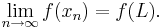
An example of a discontinuous function is the function f defined by f(x) = 1 if x > 0, f(x) = 0 if x ≤ 0. Pick for instance ε = ½. There is no δ-neighborhood around x = 0 that will force all the f(x) values to be within ε of f(0). Intuitively we can think of this type of discontinuity as a sudden jump in function values.
Another example of a discontinuous function is the signum or sign function.
A more complicated example of a discontinuous function is Thomae's function.
The function

$f(x)=\begin{cases} 0\mbox{ if }x \in \mathbb{R} \setminus \mathbb{Q}\\ x\mbox{ if }x \in \mathbb{Q} \end{cases}$

is continuous at only one point, namely x = 0.

Facts about continuous functions

If two functions f and g are continuous, then f + g and fg are continuous. If g(x) ≠ 0 for all x in the domain, then f/g is also continuous.

The composition f o g of two continuous functions is continuous.

If a function is differentiable at some point c of its domain, then it is also continuous at c. The converse is not true: a function that's continuous at c need not be differentiable there. Consider for instance the absolute value function at c = 0.

Intermediate value theorem

The intermediate value theorem is an existence theorem, based on the real number property of completeness, and states:

If the real-valued function f is continuous on the closed interval [a, b] and k is some number between f(a) and f(b), then there is some number c in [a, b] such that f(c) = k.

For example, if a child grows from 1m to 1.5m between the ages of 2 years and 6 years, then, at some time between 2 years and 6 years of age, the child's height must have been 1.25m.

As a consequence, if f is continuous on [a, b] and f(a) and f(b) differ in sign, then, at some point c in [a, b], f(c) must equal zero.

Extreme value theorem

The extreme value theorem states that if a function f is defined on a closed interval [a,b] (or any closed and bounded set) and is continuous there, then the function attains its maximum, i.e. there exists c ∈ [a,b] with f(c) ≥ f(x) for all x ∈ [a,b]. The same is true of the minimum of f. These statements are not, in general, true if the function is defined on an open interval (a,b) (or any set that is not both closed and bounded), as, for example, the continuous function f(x) = 1/x, defined on the open interval (0,1), does not attain a maximum, being unbounded above.

Directional continuity

A function may happen to be continuous in only one direction, either from the "left" or from the "right". A right-continuous function is a function which is continuous at all points when approached from the right. Technically, the formal definition is similar to the definition above for a continuous function but modified as follows:

The function $f$ is said to be right-continuous at the point c if and only if the following holds: For any number ε > 0 however small, there exists some number δ > 0 such that for all x in the domain with c < x < c + δ, the value of f(x) will satisfy

$f(c) - \varepsilon < f(x) < f(c) + \varepsilon.\,$

Likewise a left-continuous function is a function which is continuous at all points when approached from the left.

A function is continuous if and only if it is both right-continuous and left-continuous.

Continuous functions between metric spaces

Now consider a function f from one metric space (X, d_X) to another metric space (Y, d_Y). Then f is continuous at the point c in X if for any positive real number ε, there exists a positive real number δ such that all x in X satisfying d_X(x, c) < δ will also satisfy d_Y(f(x), f(c)) < ε.

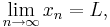
This can also be formulated in terms of sequences and limits: the function f is continuous at the point c if for every sequence (x_n) in X with limit lim x_n = c, we have lim f(x_n) = f(c). Continuous functions transform limits into limits.

This latter condition can be weakened as follows: f is continuous at the point c if and only if for every convergent sequence (x_n) in X with limit c, the sequence (f(x_n)) is a Cauchy sequence, and c is in the domain of f. Continuous functions transform convergent sequences into Cauchy sequences.

The set of points at which a function between metric spaces is continuous is a G_δ set – this follows from the ε-δ definition of continuity.

Continuous functions between topological spaces

Main article: Continuous function (topology)

The above definitions of continuous functions can be generalized to functions from one topological space to another in a natural way; a function f : X → Y, where X and Y are topological spaces, is continuous if and only if for every open set V ⊆ Y, the inverse image

$f^{-1}(V) = \{x \in X \; | \; f(x) \in V \}$

is open.

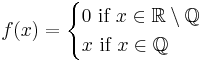
However, this definition is often difficult to use directly. Instead, suppose we have a function f from X to Y, where X,Y are topological spaces. We say f is continuous at x for some $x \in X$ if for any neighborhood V of f(x), there is a neighborhood U of x such that $f(U) \subseteq V$ . Although this definition appears complex, the intuition is that no matter how "small" V becomes, we can always find a U containing x that will map inside it. If f is continuous at every $x \in X$ , then we simply say f is continuous.

In a metric space, it is equivalent to consider the neighbourhood system of open balls centered at x and f(x) instead of all neighborhoods. This leads to the standard ε-δ definition of a continuous function from real analysis, which says roughly that a function is continuous if all points close to x map to points close to f(x). This only really makes sense in a metric space, however, which has a notion of distance.

Note, however, that if the target space is Hausdorff, it is still true that f is continuous at a if and only if the limit of f as x approaches a is f(a). At an isolated point, every function is continuous.

Continuous functions between partially ordered sets

In order theory, continuity of a function between posets is Scott continuity. Let X be a complete lattice, then a function f : X → X is continuous if, for each subset Y of X, we have sup f(Y) = f(sup Y).

Continuous binary relation

A binary relation R on A is continuous if R(a, b) whenever there are sequences (a^k)_i and (b^k)_i in A which converge to a and b respectively for which R(a^k, b^k) for all k. Clearly, if one treats R as a characteristic function in two variables, this definition of continuous is identical to that for continuous functions.

Notes

↑ "Heine continuity implies Cauchy continuity without the Axiom of Choice". Apronus.com.

References

Visual Calculus by Lawrence S. Husch, University of Tennessee (2001)