Chebyshev's inequality

In probability theory, Chebyshev's inequality (also known as Tchebysheff's inequality, Chebyshev's theorem, or the Bienaymé-Chebyshev inequality) states that in any data sample or probability distribution, nearly all the values are close to the mean value, and provides a quantitative description of "nearly all" and "close to".

In particular,

No more than 1/4 of the values are more than 2 standard deviations away from the mean;
No more than 1/9 are more than 3 standard deviations away;
No more than 1/25 are more than 5 standard deviations away;

and so on. In general:

No more than 1/k² of the values are more than k standard deviations away from the mean.

Chebyshev's inequality is named for the Russian mathematician Pafnuty Chebyshev, although it was first formulated by his friend and colleague Irénée-Jules Bienaymé.^[1]

1 General statement
2 Variant: One-sided Chebyshev inequality
3 Proof (of the two-sided Chebyshev's inequality)
- 3.1 Measure-theoretic proof
- 3.2 Probabilistic proof
4 See also
5 References
6 Further reading

General statement

The inequality can be stated quite generally using measure theory; the statement in the language of probability theory then follows as a particular case, for a space of measure 1.

Measure-theoretic statement

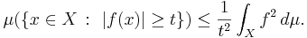
Let (X,Σ,μ) be a measure space, and let f be an extended real-valued measurable function defined on X. Then for any real number t > 0,

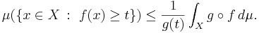
$\mu(\{x\in X\,:\,\,|f(x)|\geq t\}) \leq {1\over t^2} \int_X f^2 \, d\mu.$

More generally, if g is a nonnegative extended real-valued measurable function, nondecreasing on the range of f, then

$\mu(\{x\in X\,:\,\,f(x)\geq t\}) \leq {1\over g(t)} \int_X g\circ f\, d\mu.$

The previous statement then follows by defining g(t) as

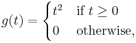
$g(t)=\begin{cases}t^2&\mbox{if }t\geq0\\0&\mbox{otherwise,}\end{cases}$

and taking |f| instead of f.

Probabilistic statement

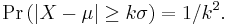
Let X be a random variable with expected value μ and finite variance σ². Then for any real number k > 0,

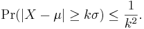
$\Pr(\left|X-\mu\right|\geq k\sigma)\leq\frac{1}{k^2}.$

Only the cases k > 1 provide useful information. This can be equivalently stated as

$\Pr(\left|X-\mu\right|\geq \alpha)\leq\frac{\sigma^2}{\alpha^2}.$

As an example, using k = √2 shows that at least half of the values lie in the interval (μ − √2 σ, μ + √2 σ).

Typically, the theorem will provide rather loose bounds. However, the bounds provided by Chebyshev's inequality cannot, in general (remaining sound for variables of arbitrary distribution), be improved upon. For example, for any k > 1, the following example (where σ = 1/k) meets the bounds exactly.

$\begin{align} & \Pr(X=-1) = 1/(2k^2), \\ \\ & \Pr(X=0) = 1 - 1/k^2, \\ \\ & \Pr(X=1) = 1/(2k^2). \end{align}$

For this distribution,

$\mathrm{Pr}\left(\left|X-\mu\right| \ge k\sigma\right) = 1/k^2.\,$

Equality holds exactly for any distribution that is a linear transformation of this one. Inequality holds for any distribution that is not a linear transformation of this one.

The theorem can be useful despite loose bounds because it applies to random variables of any distribution, and because these bounds can be calculated knowing no more about the distribution than the mean and variance.

Chebyshev's inequality is used for proving the weak law of large numbers.

Example

For illustration, assume we have a large body of text, for example articles from a publication. Assume we know that the articles are on average 1000 characters long with a standard deviation of 200 characters. From Chebyshev's inequality we can then infer that the chance that a given article is between 600 and 1400 characters would be at least 75% (k = 2).

The inequality is coarse: a more accurate guess would be possible if the distribution of the length of the articles is known. For example, a normal distribution would yield a 75% chance of an article being between 770 and 1230 characters long.

Variant: One-sided Chebyshev inequality

A one-tailed variant with k > 0, is^[2]

$\Pr(X-\mu \geq k\sigma)\leq\frac{1}{1+k^2}.$

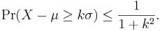
The one-sided version of the Chebyshev inequality is called Cantelli's inequality, and is due to Francesco Paolo Cantelli.

Proof (of the two-sided Chebyshev's inequality)

Measure-theoretic proof

Let $~A_t$ be defined as $A_t�:= \{x \in X \mid f(x) \geq t\}$ , and let $1_{A_t}$ be the indicator function of the set $~A_t$ . Then, it is easy to check that

$0\leq g(t) 1_{A_t}\leq g\circ f\,1_{A_t}\leq g\circ f,$

and therefore,

$g(t)\mu(A_t)=\int_X g(t)1_{A_t}\,d\mu\leq\int_{A_t} g\circ f\,d\mu\leq\int_X g\circ f\,d\mu.$

The desired inequality follows from dividing the above inequality by g(t).

Probabilistic proof

Markov's inequality states that for any real-valued random variable Y and any positive number a, we have Pr(|Y| > a) ≤ E(|Y|)/a. One way to prove Chebyshev's inequality is to apply Markov's inequality to the random variable Y = (X − μ)² with a = (σk)².

It can also be proved directly. For any event A, let I_A be the indicator random variable of A, i.e. I_A equals 1 if A occurs and 0 otherwise. Then

$\Pr(|X-\mu| \geq k\sigma) = \operatorname{E}(I_{|X-\mu| \geq k\sigma}) = \operatorname{E}(I_{[(X-\mu)/(k\sigma)]^2 \geq 1})$

$\leq \operatorname{E}\left( \left( {X-\mu \over k\sigma} \right)^2 \right) = {1 \over k^2} {\operatorname{E}((X-\mu)^2) \over \sigma^2} = {1 \over k^2}.$

The direct proof shows why the bounds are quite loose in typical cases: the number 1 to the left of "≥" is replaced by [(X − μ)/(kσ)]² to the right of "≥" whenever the latter exceeds 1. In some cases it exceeds 1 by a very wide margin.

References

↑ Donald Knuth, "The Art of Computer Programming", 3rd edition, volume 1, 1997, p.76
↑ Grimmett and Stirzaker, problem 7.11.9. Several proofs of this result can be found here.