Characteristic function (probability theory)

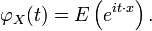
In probability theory, the characteristic function of any random variable completely defines its probability distribution. On the real line it is given by the following formula, where X is any random variable with the distribution in question:

$\varphi_X(t) = \operatorname{E}\left(e^{itX}\right)\,$

where t is a real number, i is the imaginary unit, and E denotes the expected value.

If F_X is the cumulative distribution function, then the characteristic function is given by the Riemann-Stieltjes integral

$\operatorname{E}\left(e^{itX}\right) = \int_{-\infty}^{\infty} e^{itx}\,dF_X(x).\,$

In cases in which there is a probability density function, f_X, this becomes

$\operatorname{E}\left(e^{itX}\right) = \int_{-\infty}^{\infty} e^{itx} f_X(x)\,dx.$

If X is a vector-valued random variable, one takes the argument t to be a vector and tX to be a dot product.

Every probability distribution on R or on Rⁿ has a characteristic function, because one is integrating a bounded function over a space whose measure is finite, and for every characteristic function there is exactly one probability distribution.

The characteristic function of a symmetric PDF (that is, one with $p(x)=p(-x)$ ) is real, because the imaginary components obtained from $x>0$ cancel those from $x<0$ .

1 Lévy continuity theorem
2 The inversion theorem
3 Bochner-Khinchin theorem
4 Uses of characteristic functions
5 Multivariate characteristic functions
- 5.1 Example
6 Matrix-valued random variables
7 Related concepts
8 References

Lévy continuity theorem

Main article: Lévy continuity theorem

The core of the Lévy continuity theorem states that a sequence of random variables $\scriptstyle (X_n)_{n=1}^\infty$ where each $\scriptstyle X_n$ has a characteristic function $\scriptstyle \varphi_n$ will converge in distribution towards a random variable $\scriptstyle X$ ,

$X_n \xrightarrow{\mathcal D} X \qquad\textrm{as}\qquad n \to \infty$

$\varphi_n \quad \xrightarrow{\textrm{pointwise}} \quad \varphi \qquad\textrm{as}\qquad n \to \infty$

and $\scriptstyle \varphi(t)$ continuous in $\scriptstyle t=0$ and $\scriptstyle \varphi$ is the characteristic function of $\scriptstyle X$ .

The Lévy continuity theorem can be used to prove the weak law of large numbers, see the proof using convergence of characteristic functions.

The inversion theorem

There is a bijection between cumulative probability distribution functions and characteristic functions. In other words, two distinct probability distributions never share the same characteristic function.

Given a characteristic function φ, it is possible to reconstruct the corresponding cumulative probability distribution function F:

$F_X(y) - F_X(x) = \lim_{\tau \to +\infty} \frac{1} {2\pi} \int_{-\tau}^{+\tau} \frac{e^{-itx} - e^{-ity}} {it}\, \varphi_X(t)\, dt.$

In general this is an improper integral; the function being integrated may be only conditionally integrable rather than Lebesgue integrable, i.e. the integral of its absolute value may be infinite.

Reference: see (P. Levy, Calcul des probabilites, Gauthier-Villars, Paris, 1925. p166)

Bochner-Khinchin theorem

Main article: Bochner's theorem

An arbitrary function $\scriptstyle \varphi$ is a characteristic function corresponding to some probability law $\scriptstyle \mu$ if and only if the following three conditions are satisfied:

(1) $\scriptstyle \varphi \,$ is continuous

(2) $\scriptstyle \varphi(0) = 1 \,$

(3) $\scriptstyle \varphi \,$ is a positive definite function (note that this is a complicated condition which is not equivalent to $\scriptstyle \varphi >0$ ).

Uses of characteristic functions

Because of the continuity theorem, characteristic functions are used in the most frequently seen proof of the central limit theorem. The main trick involved in making calculations with a characteristic function is recognizing the function as the characteristic function of a particular distribution.

Basic properties

Characteristic functions are particularly useful for dealing with functions of independent random variables. For example, if X₁, X₂, ..., X_n is a sequence of independent (and not necessarily identically distributed) random variables, and

$S_n = \sum_{i=1}^n a_i X_i,\,\!$

where the a_i are constants, then the characteristic function for S_n is given by

$\varphi_{S_n}(t)=\varphi_{X_1}(a_1t)\varphi_{X_2}(a_2t)\cdots \varphi_{X_n}(a_nt). \,\!$

In particular, $\varphi_{X+Y}(t) = \varphi_X(t)\varphi_Y(t)$ . To see this, write out the definition of characteristic function:

$\varphi_{X+Y}(t)=E\left(e^{it(X+Y)}\right)=E\left(e^{itX}e^{itY}\right)=E\left(e^{itX}\right)E\left(e^{itY}\right)=\varphi_X(t) \varphi_Y(t)$ .

Observe that the independence of $X$ and $Y$ is required to establish the equality of the third and fourth expressions.

Another special case of interest is when $a_i=1/n$ and then $S_n$ is the sample mean. In this case, writing $\overline{X}$ for the mean,

$\varphi_{\overline{X}}(t)=\left(\varphi_X(t/n)\right)^n.$

Moments

Characteristic functions can also be used to find moments of a random variable. Provided that the n^th moment exists, characteristic function can be differentiated n times and

$\operatorname{E}\left(X^n\right) = i^{-n}\, \varphi_X^{(n)}(0) = i^{-n}\, \left[\frac{d^n}{dt^n} \varphi_X(t)\right]_{t=0}. \,\!$

For example, suppose $X$ has a standard Cauchy distribution. Then $\varphi_X(t)=e^{-|t|}$ . See how this is not differentiable at $t=0$ , showing that the Cauchy distribution has no expectation. Also see that the characteristic function of the sample mean $\overline{X}$ of $n$ independent observations has characteristic function $\varphi_{\overline{X}}(t)=(e^{-|t|/n})^n=e^{-|t|}$ , using the result from the previous section. This is the characteristic function of the standard Cauchy distribution: thus, the sample mean has the same distribution as the population itself.

The logarithm of a characteristic function is a cumulant generating function, which is useful for finding cumulants.

An example

The Gamma distribution with scale parameter θ and a shape parameter k has the characteristic function

$(1 - \theta\,i\,t)^{-k}.$

Now suppose that we have

$X ~\sim \Gamma(k_1,\theta) \mbox{ and } Y \sim \Gamma(k_2,\theta)$

with X and Y independent from each other, and we wish to know what the distribution of X + Y is. The characteristic functions are

$\varphi_X(t)=(1 - \theta\,i\,t)^{-k_1},\,\qquad \varphi_Y(t)=(1 - \theta\,i\,t)^{-k_2}$

which by independence and the basic properties of characteristic function leads to

$\varphi_{X+Y}(t)=\varphi_X(t)\varphi_Y(t)=(1 - \theta\,i\,t)^{-k_1}(1 - \theta\,i\,t)^{-k_2}=\left(1 - \theta\,i\,t\right)^{-(k_1+k_2)}.$

This is the characteristic function of the gamma distribution scale parameter θ and shape parameter k₁ + k₂, and we therefore conclude

$X+Y \sim \Gamma(k_1+k_2,\theta) \,$

The result can be expanded to n independent gamma distributed random variables with the same scale parameter and we get

$\forall i \in \{1,\ldots, n\}�: X_i \sim \Gamma(k_i,\theta) \qquad \Rightarrow \qquad \sum_{i=1}^n X_i \sim \Gamma\left(\sum_{i=1}^nk_i,\theta\right).$

Multivariate characteristic functions

If $X$ is a multivariate PDF, then its characteristic function is defined as

$\varphi_X(t)=E\left(e^{it\cdot x}\right).$

Here, the dot signifies vector dot product ( $t$ is in the dual space of $x$ ).

Example

If $X\sim N(0,\Sigma)$ is a multivariate Gaussian with zero mean, then

$\varphi_X(t)=E\left(e^{it\cdot x}\right) =\int_{x\in R^n}\frac{1}{\left|2\pi\Sigma\right|^{1/2}}e^{-\frac{1}{2}x^T\Sigma^{-1}x}\cdot e^{it\cdot x}dx=e^{-\frac{1}{2}t^T\Sigma t}.$

Matrix-valued random variables

If $X$ is a matrix-valued PDF, then the characteristic function is

$\varphi_X(T)=E\left(e^{i\, \mathrm{Tr}(XT)}\right)$

Here $\mathrm{Tr}(\cdot)$ is the trace function and matrix multiplication (of $T$ and $X$ ) is used. Note that the order of the multiplication is immaterial ( $XT\neq TX$ but $tr(XT)=tr(TX)$ ).

Examples of matrix-valued PDFs include the Wishart distribution.

Related concepts

Related concepts include the moment-generating function and the probability-generating function. The characteristic function exists for all probability distributions. However this is not the case for moment generating function.

The characteristic function is closely related to the Fourier transform: the characteristic function of a probability density function $p(x)$ is the complex conjugate of the continuous Fourier transform of $p(x)$ (according to the usual convention; see [1]).

$\varphi_X(t) = \langle e^{itX} \rangle = \int_{-\infty}^{\infty} e^{itx}p(x)\, dx = \overline{\left( \int_{-\infty}^{\infty} e^{-itx}p(x)\, dx \right)} = \overline{P(t)},$

where $P(t)$ denotes the continuous Fourier transform of the probability density function $p(x)$ . Likewise, $p(x)$ may be recovered from $\varphi_X(t)$ through the inverse Fourier transform:

$p(x) = \frac{1}{2\pi} \int_{-\infty}^{\infty} e^{itx} P(t)\, dt = \frac{1}{2\pi} \int_{-\infty}^{\infty} e^{itx} \overline{\varphi_X(t)}\, dt.$

Indeed, even when the random variable does not have a density, the characteristic function may be seen as the Fourier transform of the measure corresponding to the random variable.

References

Lukacs E. (1970) Characteristic Functions. Griffin, London. pp. 350
Bisgaard, T. M., Sasvári, Z. (2000) Characteristic Functions and Moment Sequences, Nova Science

Theory of probability distributions

probability mass function (pmf) · probability density function (pdf) · cumulative distribution function (cdf) · quantile function

raw moment · central moment · mean · variance · standard deviation · skewness · kurtosis

moment-generating function (mgf) · characteristic function · probability-generating function (pgf) · cumulant