Centripetal force

For the reaction to centripetal force due to Newton's law of reaction , see Reactive centrifugal force.

Figure 1: A simple example corresponding to uniform circular motion. A ball is tethered to a rotational axis and is rotating counterclockwise around the specified path at a constant angular rate ω. The velocity of the ball is a vector tangential to the orbit, and is continuously changing direction, a change requiring a radially inward directed centripetal force. The centripetal force is provided by the tether, which is in a state of tension.

The centripetal force is the external force required to make a body follow a curved path.^[1]^[2] Hence centripetal force is a kinematic force requirement, not a particular kind of force like gravity or electromagnetism. Isaac Newton's description is found in the Principia.^[3] Many different examples are examined, one being the following:

If a body revolves in an ellipsis; it is proposed to find the law of the centripetal force tending to the centre of the ellipsis.

– Isaac Newton (1687) PROPOSITION X. PROBLEM V.

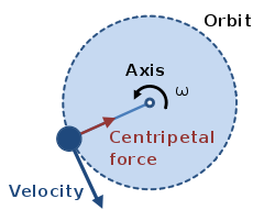
Any force (gravitational, electromagnetic, etc.) or combination of forces can act to provide a centripetal force. An example for the case of uniform circular motion is shown in Figure 1.

Centripetal force is directed inward, toward the center of curvature of the path. The term centripetal force comes from the Latin words centrum ("center") and petere ("tend towards", "aim at"), and can also be derived from Newton's original definitions described in the Principia.

Centripetal force should not be confused with centrifugal force (see the Common misunderstandings section below).

1 Simple example: uniform circular motion
2 Source of centripetal force
3 Common misunderstandings
4 Analysis of several cases
5 Notes and references
6 Further reading
7 External links
8 See also

Simple example: uniform circular motion

The velocity vector is defined by the speed and the direction of motion. Objects experiencing no net force do not accelerate and hence move in a straight line with constant speed; they have a constant velocity. However, an object moving in a circle, even at constant speed, has a changing direction of motion. The rate of change of the object's velocity vector in this case is the centripetal acceleration. See Figure 1.

The centripetal acceleration varies with the radius $R$ of the path and speed $v$ of the object, becoming larger for greater speeds (at constant radius) and smaller radii (at constant speed). If an object is traveling in a circle with a varying speed, its acceleration can be divided into two components, a radial acceleration (the centripetal acceleration that changes the direction of the velocity) and a tangential acceleration that changes the magnitude of the velocity.

Below a number of examples of increasing complexity are discussed, and formulas for the motion are derived.

Source of centripetal force

Centripetal force is inferred from the trajectory of the object, without regard for how the path was arrived at (regardless of the origin of the forces involved). The studies of trajectories and the forces they imply is kinematics, while the study of which motions result from given physical forces is kinetics, the other branch of dynamics.

Supposing the analysis of a trajectory (kinematics) has concluded that for an object to follow the observed path a centripetal force is required, one might reasonably ask the (kinetic) question: "Where is the centripetal force coming from?"

For a satellite in orbit around a planet, the centripetal force is supplied by the gravitational attraction between the satellite and the planet, and acts toward the center of mass of the two objects. For an object at the end of a rope rotating about a vertical axis, the centripetal force is the horizontal component of the tension of the rope, which acts towards the center of mass between the axis of rotation and the rotating object. For a spinning object, internal tensile stress is the centripetal force that holds the object together in one piece.

Common misunderstandings

Centripetal force should not be confused with centrifugal force. Centripetal force is a kinematic force requirement deduced from an observed trajectory, not a kinetic force like gravity or electrical forces. Centripetal force requirements may be deduced from a trajectory in any frame of reference (although the trajectory of an object and the deduced centripetal force will vary from one frame to another). Because centripetal force is a kinematic force requirement inferred from an established trajectory, it is not used to deduce a trajectory from a physical situation, and centripetal force is not included in the inventory of forces that are used in applying Newton's laws F != m a to calculate a trajectory.

Centrifugal force, on the other hand, is treated in a rotating frame as a kinetic force, that is, as part of the inventory of forces used in Newton's laws to predict motion. Centrifugal force is a fictitious force, however, that arises only when motion is described or experienced in a rotating reference frame, and it does not exist in an inertial frame of reference.^[4]

Centripetal force should not be confused with central force, either. To iterate, centripetal force is not a force requirement necessary for a curved trajectory to be possible: it is not a type of force, such as a nuclear or gravitational force. In contrast, central forces does refer to a type of force, more exactly to a class of physical forces between two objects that meet two conditions: (1) their magnitude depends only on the distance between the two objects and (2) their direction points along the line connecting the centers of these two objects. Examples of central forces include the gravitational force between two masses and the electrostatic force between two charges.

As an example relating these terms, the centripetal force implied by the circular motion of an object often is provided by a central force.

Analysis of several cases

Below are three examples of increasing complexity, with derivations of the formulas governing velocity and acceleration.

Uniform circular motion

See also: Circular motion and Uniform circular motion

Uniform circular motion refers to the case of constant rate of rotation. Here are two approaches to describing this case.

Geometric derivation

Figure 2: Left circle: The particle's orbit – particle moves in a circle and velocity is tangent to orbit; Right circle: a "velocity circle"; velocity vectors are brought together so tails coincide: because velocity is a constant in uniform motion, the tip of the velocity vector describes a circle, and acceleration is tangent to the velocity circle. That means the acceleration is radially inward in the left-hand circle showing the orbit.

The circle on the left in Figure 2 shows an object moving on a circle at constant speed at two different times in its orbit. Its position is given by R and its velocity is v.

The velocity vector v is always perpendicular to the position vector (since the velocity vector is always tangent to the R circle); thus, since R moves in a circle, so does v. The circular motion of the velocity is shown in the circle on the right of Figure 2, along with its acceleration a. Just as velocity is the rate of change of position, acceleration is the rate of change of velocity.

Since the position and velocity vectors move in tandem, they go around their circles in the same time T. That time equals the distance traveled divided by the velocity

$T = \frac{2\pi R}{v}$

and, by analogy,

$T = \frac{2\pi v}{a}$

Setting these two equations equal and solving for $a$ , we get

$a = \frac{v^{2}}{R}$

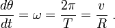
The angular rate of rotation in radians / s is:

$\omega = \frac {2 \pi} {T} \$

Comparing the two circles in Figure 2 also shows that the acceleration points toward the center of the R circle. For example, in the left circle in Figure 2, the position vector R pointing at 12 o'clock has a velocity vector v pointing at 9 o'clock, which (switching to the circle on the right) has an acceleration vector a pointing at 6 o'clock. So the acceleration vector is opposite to R and toward the center of the R circle.

Derivation using vectors

Figure 3: Vector relationships for uniform circular motion; vector Ω representing the rotation is normal to the plane of the orbit with polarity determined by the right-hand rule and magnitude dθ /dt.

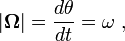
Figure 3 shows the vector relationships for uniform circular motion. The rotation itself is represented by the vector Ω, which is normal to the plane of the orbit (using the right-hand rule) and has magnitude given by:

$\left| \boldsymbol {\Omega}\right| = \frac {d \theta } {dt} = \omega \ ,$

with θ the angular position at time t. In this subsection, dθ / dt is assumed constant, independent of time t. The displacement of the particle in time dt along the circular path is

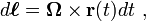
$d\boldsymbol{\ell} = \boldsymbol {\Omega} \times \mathbf{r} ( t ) dt \ ,$

which, by properties of the vector cross product, has magnitude r d θ and is in the direction tangent to the circular path.

Consequently,

$\frac {d \mathbf{r}}{dt} = \frac {\mathbf{r}(t + dt)-\mathbf{r}(t )}{dt} = \frac{d \boldsymbol{\ell}}{dt} \ .$

In other words,

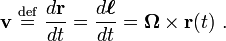
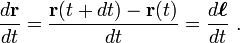
$\mathbf{v}\ \stackrel{\mathrm{def}}{=}\ \frac {d \mathbf{r}}{dt} = \frac {d\boldsymbol{\ell}}{dt} = \boldsymbol {\Omega} \times \mathbf{r} ( t )\ .$

Differentiating with respect to time,

$\mathbf{a}\ \stackrel{\mathrm{def}}{=}\ \frac {d \mathbf{v}} {dt} = \boldsymbol {\Omega} \times \frac{d \mathbf{r} ( t )}{dt} = \boldsymbol {\Omega} \times \left[ \boldsymbol {\Omega} \times \mathbf{r} (t)\right] \ .$

Lagrange's formula states:

a × (b × c) = b(a · c) − c(a · b).

Applying Lagrange's formula with the observation that Ω • r (t) = 0 at all times,

$\mathbf{a} = - {\Omega}^2 \mathbf{r} (t) \ .$

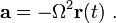
In words, the acceleration is pointing directly opposite to the radial displacement r at all times, and has a magnitude:

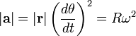
$|\mathbf{a}| = |\mathbf{r}| \left ( \frac {d \theta}{dt} \right) ^2 = R {\omega}^2\$

where vertical bars |…| denote the vector magnitude, which in the case of r(t) is simply the radius R of the path. This result agrees with the previous section if the substitution is made for rate of rotation in terms of the period of rotation T:

$\frac {d \theta }{dt} = \omega = \frac {2 \pi } {T} = \frac {v}{R} \ .$

Not surprisingly, this result also agrees with that of the nonuniform circular motion when the rate of rotation is made constant.

A merit of the vector approach is that it is manifestly independent of any coordinate system.

Example: The banked turn

Main article: Banked turn

See also: Reactive centrifugal force#Example: The turning car

Figure 4: Left panel: Ball on a banked circular track moving with constant speed v; Right panel: Forces on the ball. The resultant or net force on the ball found by vector addition of the normal force exerted by the road and vertical force due to gravity must equal the centripetal force dictated by the need to travel a circular path.

Figure 4 shows a ball in circular motion on a banked curve. The curve is banked at an angle θ from the horizontal, and the surface of the road is considered to be slippery. The object is to find what angle θ the bank must have so the ball does not slide off the road (the so-called "angle of bank").^[5] Intuition tells us that on a flat curve with no banking at all, the ball will simply slide off the road; while with a very steep banking, the ball will slide to the center unless it travels the curve rapidly.

The right side of Figure 4 indicates the forces on the ball. There are two forces; one is the force of gravity vertically downward through the center of mass of the ball m g where m is the mass of the ball and g is the gravitational acceleration; the second is the upward normal force exerted by the road perpendicular to the road surface m a_n. The centripetal force shown in Figure 4 is the net force obtained by vector addition of the normal force and the force of gravity, and is not a third force applied to the ball.

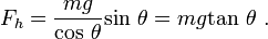
The horizontal net force on the ball is the horizontal component of the force from the road, which has magnitude F_h = m a_n sin θ. The vertical component of the force from the road must counteract the gravitational force, that is F_v = m a_n cos θ = m g, so m a_n = m g / cos θ. Accordingly one finds the net horizontal force to be:

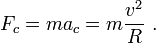
$F_h = \frac {m g } { \mathrm{cos}\ \theta} \mathrm {sin}\ \theta = mg \mathrm{tan}\ \theta \ .$

On the other hand, at velocity v on a circular path of radius R, kinematics says that the force needed to turn the ball continuously into the turn is the radially inward centripetal force F_c of magnitude:

$F_c = m a _c = m\frac{v^2}{R} \ .$

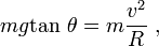
Consequently the ball is in a stable path when the angle of the road is set to satisfy the condition:

$mg \mathrm{tan}\ \theta = m\frac{v^2}{R} \ ,$

or,

$\mathrm{tan}\ \theta = \frac {v^2} {gR} \ .$

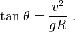
As the angle of bank θ approaches 90°, the tangent function approaches infinity, allowing larger values for v² / R. In words, this equation states that for faster speeds (bigger v) the road must be banked more steeply (a larger value for θ), and for sharper turns (smaller R) the road also must be banked more steeply, which accords with intuition. When the angle θ does not satisfy the above condition, the horizontal component of force exerted by the road does not provide the correct centripetal force, and an additional frictional force tangential to the road surface is called upon to provide the difference.^[6] If friction cannot do this (that is, the coefficient of friction is exceeded), the ball slides to a different radius where the balance can be realized.^[7]^[8]

These ideas apply to air flight as well. See the FAA pilot's manual.^[9]

Nonuniform circular motion

See also: Circular motion and Non-uniform circular motion

Figure 5: Velocity and acceleration for nonuniform circular motion: the velocity vector is tangential to the orbit, but the acceleration vector is not radially inward because of its tangential component a_θ that increases the rate of rotation: dω / dt = | a_θ | / R.

As a generalization of the uniform circular motion case, suppose the angular rate of rotation is not constant. The acceleration now has a tangential component, as shown in Figure 5. This case is used to demonstrate a derivation strategy based upon a polar coordinate system.

Let r(t) be a vector that describes the position of a point mass as a function of time. Since we are assuming circular motion, let r(t) = R·u_r, where R is a constant (the radius of the circle) and u_r is the unit vector pointing from the origin to the point mass. The direction of u_r is described by θ, the angle between the x-axis and the unit vector, measured counterclockwise from the x-axis. The other unit vector for polar coordinates, u_θ is perpendicular to u_r and points in the direction of increasing θ. These polar unit vectors can be expressed in terms of Cartesian unit vectors in the x and y directions, denoted i and j respectively:

u_r = cos(θ) i + sin(θ) j

and

u_θ = sin(θ) i + cos(θ) j.

Note: unlike the Cartesian unit vectors i and j, which are constant, in polar coordinates the direction of the unit vectors u_r and u_θ depend on θ, and so in general have non-zero time derivatives.

We differentiate to find velocity:

$\mathbf{v} = R \frac {d \mathbf{u_r}}{dt} = R \frac {d}{dt} \left( \mathrm{cos}\ \theta \ \mathbf{i} + \mathrm{sin}\ \theta \ \mathbf{j}\right)$

$= R \frac {d \theta} {dt} \left( -\mathrm{sin}\ \theta \ \mathbf{i} + \mathrm{cos}\ \theta \ \mathbf{j}\right)\,$

$= R \frac{d\theta}{dt} \mathbf{u_\theta} \,$

$= R \omega \mathbf{u_\theta} \,$

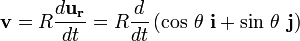
where ω is the angular velocity dθ/dt.

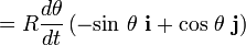
This result for the velocity matches expectations that the velocity should be directed tangential to the circle, and that the magnitude of the velocity should be ωR. Differentiating again, and noting that

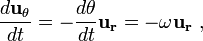
${\frac {d\mathbf{u_\theta}}{dt}} = -\frac{d\theta}{dt} \mathbf{u_r} = - \omega \mathbf{u_r} \ ,$

we find that the acceleration, a is:

$\mathbf{a} = R \left( \frac {d\omega}{dt} \mathbf{u_\theta} - \omega^2 \mathbf{u_r} \right) \ .$

Thus, the radial and tangential components of the acceleration are:

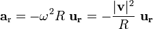$\mathbf{a}_{\mathrm{r}} = - \omega^{2} R \ \mathbf{u_r}=- \frac{|\mathbf{v}|^{2}}{ R} \ \mathbf{u_r} \$ and $\ \mathbf{a}_{\mathrm{\theta}}=R \ \frac {d\omega}{dt} \ \mathbf{u_\theta} = \frac {d | \mathbf{v} | }{dt} \ \mathbf{u_\theta} \ ,$

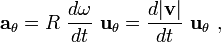
where |v| = Rω is the magnitude of the velocity (the speed).

These equations express mathematically that, in the case of an object that moves along a circular path with a changing speed, the acceleration of the body may be decomposed into a perpendicular component that changes the direction of motion (the centripetal acceleration), and a parallel, or tangential component, that changes the speed.

General planar motion

See also: Generalized forces, Generalized force, Curvilinear coordinates, Generalized coordinates, and Orthogonal coordinates

Figure 6: Polar unit vectors at two times t and t+dt for a particle with trajectory r ( t ); on the left the unit vectors u_ρ and u_θ at the two times are moved so their tails all meet, and are shown to trace an arc of a unit radius circle. Their rotation in time dt is dθ, just the same angle as the rotation of the trajectory r ( t ).

Polar coordinates

The above results can be derived perhaps more simply in polar coordinates, and at the same time extended to general motion within a plane, as shown next. Polar coordinates in the plane employ a radial unit vector u_ρ and an angular unit vector u_θ, as shown in Figure 6.^[10] A particle at position r is described by:

$\mathbf{r} = \rho \mathbf{u}_{\rho} \ ,$

where the notation ρ is used to describe the distance of the path from the origin instead of R to emphasize that this distance is not fixed, but varies with time. The unit vector u_ρ travels with the particle and always points in the same direction as r ( t ). Unit vector u_θ also travels with the particle and stays orthogonal to u_ρ. Thus, u_ρ and u_θ form a local Cartesian coordinate system attached to the particle, and tied to the path traveled by the particle.^[11] By moving the unit vectors so their tails coincide, as seen in the circle at the left of Figure 6, it is seen that u_ρ and u_θ form a right-angled pair with tips on the unit circle that trace back and forth on the perimeter of this circle with the same angle θ (t) as r ( t ).

When the particle moves, its velocity is

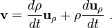
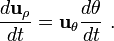
$\mathbf{v} = \frac {d \rho }{dt} \mathbf{u}_{\rho} + \rho \frac {d \mathbf{u}_{\rho}}{dt} \ .$

To evaluate the velocity, the derivative of the unit vector u_ρ is needed. Because u_ρ is a unit vector, its magnitude is fixed, and it can change only in direction, that is, its change du_ρ has a component only perpendicular to u_ρ. When the trajectory r ( t ) rotates an amount dθ, u_ρ, which points in the same direction as r ( t ), also rotates by dθ. See Figure 6. Therefore the change in u_ρ is

$d \mathbf{u}_{\rho} = \mathbf{u}_{\theta} d\theta \ ,$

$\frac {d \mathbf{u}_{\rho}}{dt} = \mathbf{u}_{\theta} \frac {d\theta}{dt} \ .$

In a similar fashion, the rate of change of u_θ is found. As with u_ρ, u_θ is a unit vector and can only rotate without changing size. To remain orthogonal to u_ρ while the trajectory r ( t ) rotates an amount dθ, u_θ, which is orthogonal to r ( t ), also rotates by dθ. See Figure 6. Therefore, the change du_θ is orthogonal to u_θ and proportional to dθ (see Figure 6):

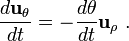
$\frac{d \mathbf{u}_{\theta}}{dt} = -\frac {d \theta} {dt} \mathbf{u}_{\rho} \ .$

Figure 6 shows the sign to be negative: to maintain orthogonality, if du_ρ is positive with d θ, then du_θ must decrease.

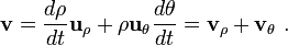
Substituting the derivative of u_ρ into the expression for velocity:

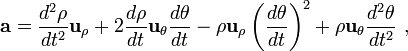
$\mathbf{v} = \frac {d \rho }{dt} \mathbf{u}_{\rho} + \rho \mathbf{u}_{\theta} \frac {d \theta} {dt} =\mathbf{v}_{\rho} + \mathbf{v}_{\theta} \ .$

To obtain the acceleration, another time differentiation is done:

$\mathbf{a} = \frac {d^2 \rho }{dt^2} \mathbf{u}_{\rho}+ \frac {d \rho }{dt} \frac{d \mathbf{u}_{\rho}}{dt} +\frac {d \rho}{dt} \mathbf{u}_{\theta} \frac {d \theta} {dt}+\rho \frac{d \mathbf{u}_{\theta}}{dt} \frac {d \theta} {dt}+\rho \mathbf{u}_{\theta} \frac {d^2 \theta} {dt^2} \ .$

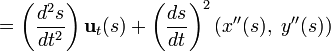
Substituting the derivatives of u_ρ and u_θ, the acceleration of the particle is:^[12]

$\mathbf{a} = \frac {d^2 \rho }{dt^2} \mathbf{u}_{\rho}+ 2\frac {d \rho}{dt} \mathbf{u}_{\theta} \frac {d \theta} {dt}-\rho \mathbf{u}_{\rho}\left( \frac {d \theta} {dt}\right)^2+\rho \mathbf{u}_{\theta} \frac {d^2 \theta} {dt^2} \ ,$

$=\mathbf{u}_{\rho} \left[ \frac {d^2 \rho }{dt^2}-\rho\left( \frac {d \theta} {dt}\right)^2 \right] + \mathbf{u}_{\theta}\left[ 2\frac {d \rho}{dt} \frac {d \theta} {dt}+\rho \frac {d^2 \theta} {dt^2}\right] \$

$=\mathbf{u}_{\rho} \left[ \frac {d|\mathbf{v}_{\rho}|}{dt}-\frac{|\mathbf{v}_{\theta}|^2}{\rho}\right] +\mathbf{u}_{\theta}\left[ \frac{2}{\rho}|\mathbf{v}_{\rho}||\mathbf{v}_{\theta}|+\rho\frac{d}{dt}\frac{|\mathbf{v}_{\theta}|}{\rho}\right] \ .$

As a particular example, if the particle moves in a circle of constant radius R, then dρ / dt = 0, v = v_θ, and:

$\mathbf{a}=\mathbf{u}_{\rho} \left[ -\rho\left( \frac {d \theta} {dt}\right)^2 \right] + \mathbf{u}_{\theta}\left[ \rho \frac {d^2 \theta} {dt^2}\right] \$

$= \mathbf{u}_{\rho} \left[ -\frac{\mathbf{v}^2}{R}\right] + \mathbf{u}_{\theta}\left[ \frac {d |\mathbf{v}|} {dt}\right] \ .$

These results agree with those above for nonuniform circular motion. See also the article on non-uniform circular motion. If this acceleration is multiplied by the particle mass, the leading term is the centripetal force and the negative of the second term related to angular acceleration is sometimes called the Euler force.^[13]

For trajectories other than circular motion, for example, the more general trajectory envisioned in Figure 6, the instantaneous center of rotation and radius of curvature of the trajectory are related only indirectly to the coordinate system defined by u_ρ and u_θ and to the length |r ( t)| = ρ. Consequently, in the general case, it is not straightforward to disentangle the centripetal and Euler terms from the above general acceleration equation.^[14] ^[15] To deal directly with this issue, local coordinates are preferable, as discussed next.

Local coordinates

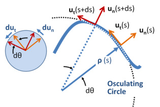
Figure 7: Local coordinate system for planar motion on a curve. Two different positions are shown for distances s and s + ds along the curve. At each position s, unit vector u_n points along the outward normal to the curve and unit vector u_t is tangential to the path. The radius of curvature of the path is ρ as found from the rate of rotation of the tangent to the curve with respect to arc length, and is the radius of the osculating circle at position s. The unit circle on the left shows the rotation of the unit vectors with s.

By local coordinates is meant a set of coordinates that travel with the particle, ^[16] and have orientation determined by the path of the particle.^[17] Unit vectors are formed as shown in Figure 7, both tangential and normal to the path. This coordinate system sometimes is referred to as intrinsic or path coordinates^[18]^[19] or nt-coordinates, for normal-tangential, referring to these unit vectors. These coordinates are a very special example of a more general concept of local coordinates from the theory of differential forms.^[20]

Distance along the path of the particle is the arc length s, considered to be a known function of time.

$s = s(t) \ .$

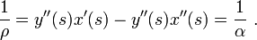
A center of curvature is defined at each position s located a distance ρ (the radius of curvature) from the curve on a line along the normal u_n (s). The required distance ρ (s) at arc length s is defined in terms of the rate of rotation of the tangent to the curve, which in turn is determined by the path itself. If the orientation of the tangent relative to some starting position is θ (s), then ρ (s) is defined by the derivative dθ / ds:

$\frac{1} {\rho (s)} =\kappa (s) = \frac {d\theta}{ds}\ .$

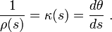
The radius of curvature usually is taken as positive (that is, as an absolute value), while the curvature κ is a signed quantity.

A geometric approach to finding the center of curvature and the radius of curvature uses a limiting process leading to the osculating circle.^[21]^[22] See Figure 7.

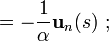
Using these coordinates, the motion along the path is viewed as a succession of circular paths of ever-changing center, and at each position s constitutes non-uniform circular motion at that position with radius ρ. The local value of the angular rate of rotation then is given by:

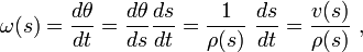
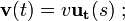
$\omega(s) = \frac{d\theta}{dt} = \frac{d\theta}{ds} \frac {ds}{dt} =\frac{1}{\rho (s)}\ \frac {ds}{dt} =\frac{v(s)}{\rho (s)}\ ,$

with the local speed v given by:

$v(s) = \frac {ds}{dt}\ .$

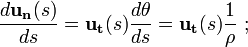
As for the other examples above, because unit vectors cannot change magnitude, their rate of change is always perpendicular to their direction (see the left-hand insert in Figure 7):^[23]

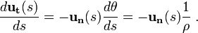
$\frac{d\mathbf{u_n}(s)}{ds} = \mathbf{u_t}(s)\frac{d\theta}{ds} = \mathbf{u_t}(s)\frac{1}{\rho} \�;$ $\frac{d\mathbf{u_t}(s)}{ds} = -\mathbf{u_n}(s)\frac{d\theta}{ds} =- \mathbf{u_n}(s)\frac{1}{\rho} \ .$

Consequently, the velocity and acceleration are:^[24]^[22]^[25]

$\mathbf{v}(t) = v \mathbf{u_t}(s)\�;$

and using the chain-rule of differentiation:

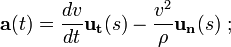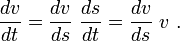
$\mathbf{a}(t) = \frac{dv}{dt} \mathbf{u_t}(s) - \frac{v^2}{\rho}\mathbf{u_n}(s) \�;$ with the tangential acceleration $\frac{dv}{dt} = \frac{dv}{ds}\ \frac{ds}{dt} =\frac{dv}{ds}\ v \ .$

In this local coordinate system the acceleration resembles the expression for nonuniform circular motion with the local radius ρ(s), and the centripetal acceleration is identified as the second term.^[26]

Extension of this approach to three dimensional space curves leads to the Frenet-Serret formulas.^[27]^[28]

Alternative approach

Looking at Figure 7, one might wonder whether adequate account has been taken of the difference in curvature between ρ(s) and ρ(s + ds) in computing the arc length as ds = ρ(s)dθ. Reassurance on this point can be found using a more formal approach outlined below. This approach also makes connection with the article on curvature.

To introduce the unit vectors of the local coordinate system, one approach is to begin in Cartesian coordinates and describe the local coordinates in terms of these Cartesian coordinates. In terms of arc length s let the path be described as:^[29]

$\mathbf{r}(s) = \left[ x(s),\ y(s) \right] \ .$

Then an incremental displacement along the path ds is described by:

$d\mathbf{r}(s) = \left[ dx(s),\ dy(s) \right]=\left[ x'(s),\ y'(s) \right] ds \ ,$

where primes are introduced to denote derivatives with respect to s. The magnitude of this displacement is ds, showing that:^[30]

$\left[ x'(s)^2 + y'(s)^2 \right] = 1 \ .$ (Eq. 1)

This displacement is necessarily tangent to the curve at s, showing that the unit vector tangent to the curve is:

$\mathbf{u}_t(s) = \left[ x'(s), \ y'(s) \right] \ ,$

while the outward unit vector normal to the curve is

$\mathbf{u}_n(s) = \left[ y'(s),\ -x'(s) \right] \ ,$

Orthogonality can be verified by showing the vector dot product is zero. The unit magnitude of these vectors is a consequence of Eq. 1. Using the tangent vector, the angle of the tangent to the curve, say θ, is given by:

$\sin \theta =\frac{y'(s)}{\sqrt{x'(s)^2+y'(s)^2}} = y'(s) \�;$ and $\cos \theta =\frac{x'(s)}{\sqrt{x'(s)^2+y'(s)^2}} = x'(s) \ .$

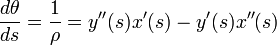
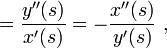
The radius of curvature is introduced completely formally (without need for geometric interpretation) as:

$\frac{1}{\rho} = \frac{d\theta}{ds}\ .$

The derivative of θ can be found from that for sin θ:

$\frac{d \sin\theta}{ds} = \cos \theta \frac {d\theta}{ds} = \frac{1}{\rho} \cos \theta \$

$= \frac{1}{\rho} x'(s)\ .$

Now:

$\frac{d \sin \theta }{ds} = \frac{d}{ds} \frac{y'(s)}{\sqrt{x'(s)^2+y'(s)^2}}$ $= \frac{y''(s)x'(s)^2-y'(s)x'(s)x''(s)} {\left(x'(s)^2+y'(s)^2\right)^{3/2}}\ ,$

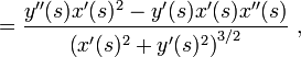
in which the denominator is unity. With this formula for the derivative of the sine, the radius of curvature becomes:

$\frac {d\theta}{ds} = \frac{1}{\rho} = y''(s)x'(s) - y'(s)x''(s)\$ $=\frac{y''(s)}{x'(s)} = -\frac{x''(s)}{y'(s)} \ ,$

where the equivalence of the forms stems from differentiation of Eq. 1:

$x'(s)x''(s) + y'(s)y''(s) = 0 \ .$

With these results, the acceleration can be found:

$\mathbf{a}(s) = \frac{d}{dt}\mathbf{v}(s)$ $= \frac{d}{dt}\left[\frac{ds}{dt} \left( x'(s), \ y'(s) \right) \right]\$

$= \left(\frac{d^2s}{dt^2}\right)\mathbf{u}_t(s) +\left(\frac{ds}{dt}\right) ^2 \left(x''(s),\ y''(s) \right)$

$= \left(\frac{d^2s}{dt^2}\right)\mathbf{u}_t(s) - \left(\frac{ds}{dt}\right) ^2 \frac{1}{\rho} \mathbf{u}_n(s) \ ,$

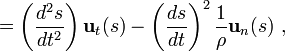
as can be verified by taking the dot product with the unit vectors u_t(s) and u_n(s). This result for acceleration is the same as that for circular motion based on the radius ρ. Using this coordinate system in the inertial frame, it is easy to identify the force normal to the trajectory as the centripetal force and that parallel to the trajectory as the tangential force. From a qualitative standpoint, the path can be approximated by an arc of a circle for a limited time, and for the limited time a particular radius of curvature applies, the centrifugal and Euler forces can be analyzed on the basis of circular motion with that radius.

This result for acceleration agrees with that found earlier. However, in this approach the question of the change in radius of curvature with s is handled completely formally, consistent with a geometric interpretation, but not relying upon it, thereby avoiding any questions Figure 7 might suggest about neglecting the variation in ρ.

Example: circular motion

To illustrate the above formulas, let x, y be given as:

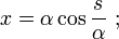
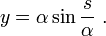
$x = \alpha \cos \frac{s}{\alpha} \�;$ $y=\alpha \sin\frac{s}{\alpha} \ .$

Then:

$x^2+y^2 = \alpha^2 \ ,$

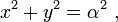
which can be recognized as a circular path around the origin with radius α. The position s = 0 corresponds to [α, 0], or 3 o'clock. To use the above formalism the derivatives are needed:

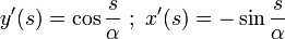
$y'(s) = \cos \frac{s}{\alpha}\�; \ x'(s) = -\sin \frac{s}{\alpha} \$

$y''(s) = -\frac{1}{\alpha}\sin\frac{s}{\alpha} \�; \ x''(s) = -\frac{1}{\alpha}\cos \frac{s}{\alpha} \ .$

With these results one can verify that:

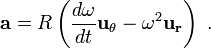
$x'(s)^2 + y'(s)^2 = 1 \$ ; $\frac{1}{\rho} = y''(s)x'(s)-y''(s)x''(s) = \frac{1}{\alpha}\ .$

The unit vectors also can be found:

$\mathbf{u}_t(s) = \left[-\sin\frac{s}{\alpha},\ \cos\frac{s}{\alpha} \right]\$ ; $\mathbf{u}_n(s) = \left[\cos\frac{s}{\alpha},\ \sin\frac{s}{\alpha} \right] \ ,$

which serve to show that s = 0 is located at position [ρ, 0] and s = ρπ/2 at [0, ρ], which agrees with the original expressions for x and y. In other words, s is measured counterclockwise around the circle from 3 o'clock. Also, the derivatives of these vectors can be found:

$\frac{d}{ds}\mathbf{u}_t(s) = -\frac{1}{\alpha} \left[\cos\frac{s}{\alpha},\ \sin\frac{s}{\alpha} \right]\$ $= -\frac{1}{\alpha}\mathbf{u}_n(s) \ �;$

$\ \frac{d}{ds}\mathbf{u}_n(s)$ $= \frac{1}{\alpha} \left[-\sin\frac{s}{\alpha},\ \cos\frac{s}{\alpha} \right]$ $= \frac{1}{\alpha}\mathbf{u}_t(s) \ .$

To obtain velocity and acceleration, a time-dependence for s is necessary. For counterclockwise motion at variable speed v(t):

$s(t) = \int_0^t \ dt' \ v(t') \ ,$

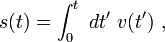
where v(t) is the speed and t is time, and s(t=0) = 0. Then:

$\mathbf{v} = v(t)\mathbf{u}_t(s) \ ,$

$\mathbf{a} = \frac{dv}{dt}\mathbf{u}_t(s)+v\frac{d}{dt}\mathbf{u}_t(s)$ $= \frac{dv}{dt}\mathbf{u}_t(s)-v\frac{1}{\alpha}\mathbf{u}_n(s)\frac{ds}{dt}$

$=\frac{dv}{dt}\mathbf{u}_t(s)-\frac{v^2}{\alpha}\mathbf{u}_n(s) \ ,$

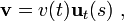
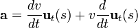
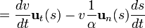
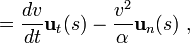
where it already is established that α = ρ. This acceleration is the standard result for non-uniform circular motion.

Notes and references

↑ Georgia State University HyperPhysics
↑ Science Joy Wagon: Centripetal force - the real force
↑ Andrew Motte translation (1729) of Newton's Principia (1687): Of the invention of Centripetal Forces, p. 114. Newton was concerned primarily with planetary motion.
↑ Inertial frames never use fictitious forces, while rotating frames must include fictitious forces that express the effects of rotation, in particular, the centrifugal force and the Coriolis force. By including fictitious forces, use of Newton's laws of motion, such as F != ma, can be extended to apply in rotating frames of reference just as well as in inertial frames of reference. Examples are provided in the article on centrifugal force.
↑ Lawrence S. Lerner (1997). Physics for Scientists and Engineers. Boston: Jones & Bartlett Publishers. p. 128. ISBN 0867204796. http://books.google.com/books?id=kJOnAvimS44C&pg=PA129&dq=centripetal+%22banked+curve%22&lr=&as_brr=0&sig=0ueAq7G5l2R3ausiXue0CPW_1dM#PPA128,M1.
↑ What is friction?
↑ Arthur Beiser (2004). Schaum's Outline of Applied Physics. New York: McGraw-Hill Professional. p. 103. ISBN 0071426116. http://books.google.com/books?id=soKguvJDgmsC&pg=PA103&dq=friction+%22banked+turn%22&lr=&as_brr=0&sig=hMYfCzJHm6Ni4Noq5v5NRvvPSyQ.
↑ Alan Darbyshire (2003). Mechanical Engineering: BTEC National Option Units. Oxford: Newnes. p. 56. ISBN 0750657618. http://books.google.com/books?id=fzfXLGpElZ0C&pg=PA57&dq=centripetal+%22banked+curve%22&lr=&as_brr=0&sig=hbaHu8Xt_uTGvd5b1DG01vCYFF8#PPA56,M1.
↑ Federal Aviation Administration (2007). Pilot's Encyclopedia of Aeronautical Knowledge. Oklahoma City OK: Skyhorse Publishing Inc.. Figure 3-21. ISBN 1602390347. http://books.google.com/books?id=m5V04SXE4zQC&pg=PT33&lpg=PT33&dq=+%22angle+of+bank%22&source=web&ots=iYTi_mZAra&sig=ytjcmr9RStdIdgZzaiBJJ-wxjts&hl=en#PPT32,M1.
↑ Although the polar coordinate system moves with the particle, the observer does not. The description of the particle motion remains a description from the stationary observer's point of view.
↑ Notice that this local coordinate system is not autonomous; for example, its rotation in time is dictated by the trajectory traced by the particle. Note also that the radial vector r ( t ) does not represent the radius of curvature of the path.
↑ John Robert Taylor (2005). Classical Mechanics. Sausalito CA: University Science Books. p. pp.28-29. ISBN 189138922X. http://books.google.com/books?id=P1kCtNr-pJsC&printsec=index&dq=isbn=189138922X&lr=&as_brr=0&source=gbs_toc_s&cad=1#PPA29,M1.
↑ Cornelius Lanczos (1986). The Variational Principles of Mechanics. New York: Courier Dover Publications. p. 103. ISBN 0486650677. http://books.google.com/books?id=ZWoYYr8wk2IC&pg=PA103&dq=%22Euler+force%22&lr=&as_brr=0&sig=UV46Q9NIrYWwn5EmYpPv-LPuZd0#PPA103,M1.
↑ See, for example, Howard D. Curtis (2005). Orbital Mechanics for Engineering Students. Butterworth-Heinemann. p. 5. ISBN 0750661690. http://books.google.com/books?id=6aO9aGNBAgIC&pg=PA193&dq=orbit+%22coordinate+system%22&lr=&as_brr=0&sig=p5hZldx_U1CnV0Ggc29YBLgLj9k#PPA5,M1.
↑ S. Y. Lee (2004). Accelerator physics (2nd Edition ed.). Hackensack NJ: World Scientific. p. 37. ISBN 981256182X. http://books.google.com/books?id=VTc8Sdld5S8C&pg=PA37&dq=orbit+%22coordinate+system%22&lr=&as_brr=0&sig=h5GU58FVOzEGclxsJkYQuVvtWkU.
↑ The observer of the motion along the curve is using these local coordinates to describe the motion from the observer's frame of reference, that is, from a stationary point of view. In other words, although the local coordinate system moves with the particle, the observer does not. A change in coordinate system used by the observer is only a change in their description of observations, and does not mean that the observer has changed their state of motion, and vice versa.
↑ Zhilin Li & Kazufumi Ito (2006). The immersed interface method: numerical solutions of PDEs involving interfaces and irregular domains. Philadelphia: Society for Industrial and Applied Mathematics. p. 16. ISBN 0898716098. http://books.google.com/books?id=_E084AX-iO8C&pg=PA16&dq=%22local+coordinates%22&lr=&as_brr=0&sig=ACfU3U2p_S2c7vRzd1vabU9WhIBJXk8ESw.
↑ K L Kumar (2003). Engineering Mechanics. New Delhi: Tata McGraw-Hill. p. 339. ISBN 0070494738. http://books.google.com/books?id=QabMJsCf2zgC&pg=PA339&dq=%22path+coordinates%22&lr=&as_brr=0&sig=ACfU3U1ZlP_syppme85cv4pimhLxyUOLug.
↑ Lakshmana C. Rao, J. Lakshminarasimhan, Raju Sethuraman & SM Sivakuma (2004). Engineering Dynamics: Statics and Dynamics. Prentice Hall of India. p. 133. ISBN 8120321898. http://books.google.com/books?id=F7gaa1ShPKIC&pg=PA134&dq=%22path+coordinates%22&lr=&as_brr=0&sig=ACfU3U0PT2mGvAHroVJFVXGB46y6zLWaGA#PPA132,M1.
↑ Shigeyuki Morita (2001). Geometry of Differential Forms. American Mathematical Society. p. 1. ISBN 0821810456. http://books.google.com/books?id=5N33Of2RzjsC&pg=PA1&dq=%22local+coordinates%22&lr=&as_brr=0&sig=ACfU3U3dnL01bMDu8d0GCmCC9eI717lsPA.
↑ The osculating circle at a given point P on a curve is the limiting circle of a sequence of circles that pass through P and two other points on the curve, Q and R, on either side of P, as Q and R approach P. See the online text by Lamb: Horace Lamb (1897). An Elementary Course of Infinitesimal Calculus. University Press. p. 406. http://books.google.com/books?id=eDM6AAAAMAAJ&pg=PA406&dq=%22osculating+circle%22&lr=&as_brr=0.
↑ ^22.0 ^22.1 Guang Chen & Fook Fah Yap (2003). An Introduction to Planar Dynamics (3rd Edition ed.). Central Learning Asia/Thomson Learning Asia. p. 34. ISBN 9812435689. http://books.google.com/books?id=xt09XiZBzPEC&pg=PA34&dq=motion+%22center+of+curvature%22&lr=&as_brr=0&sig=ACfU3U2lKY09hG88_XSHtU9H_xuaXXdGlA.
↑ R. Douglas Gregory (2006). Classical Mechanics: An Undergraduate Text. Cambridge University Press. p. 20. ISBN 0521826780. http://books.google.com/books?id=uAfUQmQbzOkC&pg=RA1-PA18&dq=particle+curve+normal+tangent&lr=&as_brr=0&sig=ACfU3U3_WR6_esuEz-mUMmOXuZabQY6Now#PRA1-PA20,M1.
↑ Edmund Taylor Whittaker & William McCrea (1988). A Treatise on the Analytical Dynamics of Particles and Rigid Bodies: with an introduction to the problem of three bodies (4rth Edition ed.). Cambridge University Press. p. 20. ISBN 0521358833. http://books.google.com/books?id=epH1hCB7N2MC&pg=PA20&vq=radius+of+curvature&dq=particle+movement+%22radius+of+curvature%22+acceleration+-soap&lr=&as_brr=0&source=gbs_search_s&sig=ACfU3U3cKHnTYJNja9o0t_Iw2VeRSGEWCg.
↑ Jerry H. Ginsberg (2007). Engineering Dynamics. Cambridge University Press. p. 33. ISBN 0521883032. http://books.google.com/books?id=je0W8N5oXd4C&pg=PA723&dq=osculating+%22planar+motion%22&lr=&as_brr=0&sig=ACfU3U0Yuca2DhshUowHlkVtw_bRSR-qww#PPA33,M1.
↑ Joseph F. Shelley (1990). 800 solved problems in vector mechanics for engineers: Dynamics. McGraw-Hill Professional. p. 47. ISBN 0070566879. http://books.google.com/books?id=ByNrVgf041MC&pg=PA46&dq=particle+movement+%22radius+of+curvature%22+acceleration+-soap&lr=&as_brr=0&sig=ACfU3U3xRX2OpTCS7_OF87Yi07fQmymg7A#PPA47,M1.
↑ Larry C. Andrews & Ronald L. Phillips (2003). Mathematical Techniques for Engineers and Scientists. SPIE Press. p. 164. ISBN 0819445061. http://books.google.com/books?id=MwrDfvrQyWYC&pg=PA164&dq=particle+%22planar+motion%22&lr=&as_brr=0&sig=ACfU3U2LpH6ofhuuC2UiED0pf38wbspY8A#PPA164,M1.
↑ Ch V Ramana Murthy & NC Srinivas (2001). Applied Mathematics. New Delhi: S. Chand & Co.. p. 337. ISBN 81-219-2082-5. http://books.google.com/books?id=Q0Pvv4vWOlQC&pg=PA337&vq=frenet&dq=isbn=8121920825&source=gbs_search_s&sig=ACfU3U3S5vGMS-NnraAEmpBf6B9bB2wK6A.
↑ The article on curvature treats a more general case where the curve is parametrized by an arbitrary variable (denoted t), rather than by the arc length s.
↑ Ahmed A. Shabana, Khaled E. Zaazaa, Hiroyuki Sugiyama (2007). Railroad Vehicle Dynamics: A Computational Approach. CRC Press. p. 91. ISBN 1420045814. http://books.google.com/books?id=YgIDSQT0FaUC&pg=RA1-PA207&dq=%22generalized+coordinate%22&lr=&as_brr=0&sig=ACfU3U2tosoLUEAUNkGu2x8TTtuxLfeLGQ#PRA1-PA91,M1.