Boundary value problem

Shows a region where a differential equation is valid and the associated boundary values

In mathematics, in the field of differential equations, a boundary value problem is a differential equation together with a set of additional restraints, called the boundary conditions. A solution to a boundary value problem is a solution to the differential equation which also satisfies the boundary conditions.

Boundary value problems arise in several branches of physics as any physical differential equation will have them. Problems involving the wave equation, such as the determination of normal modes, are often stated as boundary value problems. A large class of important boundary value problems are the Sturm-Liouville problems. The analysis of these problems involves the eigenfunctions of a differential operator.

To be useful in applications, a boundary value problem should be well posed. This means that given the input to the problem there exists a unique solution, which depends continuously on the input. Much theoretical work in the field of partial differential equations is devoted to proving that boundary value problems arising from scientific and engineering applications are in fact well-posed.

Among the earliest boundary value problems to be studied is the Dirichlet problem, of finding the harmonic functions (solutions to Laplace's equation); the solution was given by the Dirichlet principle.

1 Initial value problem
2 Types of boundary value problems
3 Example
4 See also
5 References
6 External links

Initial value problem

Main article: Initial value problem

A more mathematical way to picture the difference between an initial value problem and a boundary value problem is that an initial value problem has all of the conditions specified at the same value of the independent variable in the equation (and that value is at the lower boundary of the domain, thus the term "initial" value). On the other hand, a boundary value problem has conditions specified at the extremes of the independent variable. For example, if the independent variable is time over the domain [0,1], an initial value problem would specify a value of $y(t)$ and $y'(t)$ at time $t=0$ , while a boundary value problem would specify values for $y(t)$ at both $t=0$ and $t=1$ .

If the problem is dependent on both space and time, then instead of specifying the value of the problem at a given point for all time the data could be given at a given time for all space. For example, the temperature of an iron bar with one end kept at absolute zero and the other end at the freezing point of water would be a boundary value problem. Whereas in the middle of a still pond if somebody taps the water with a known force that would create a ripple and give us an initial condition.

Types of boundary value problems

The boundary value problem for an idealised 2D rod

If the boundary gives a value to the normal derivative of the problem then it is a Neumann boundary condition. For example, if there is a heater at one end of an iron rod, then energy would be added at a constant rate but the actual temperature would not be known.

If the boundary gives a value to the problem then it is a Dirichlet boundary condition. For example, if one end of an iron rod is held at absolute zero, then the value of the problem would be known at that point in space.

If the boundary has the form of a curve or surface that gives a value to the normal derivative and the problem itself then it is a Cauchy boundary condition.

Aside from the boundary condition, boundary value problems are also classified according to the type of differential operator involved. For an elliptic operator, one discusses elliptic boundary value problems. For an hyperbolic operator, one discusses hyperbolic boundary value problems. These categories are further subdivided into linear and various nonlinear types.

Example

For more details on Sturm-Liouville problems, for ordinary and partial differential equations, see Examples of boundary value problems.

Consider the ordinary differential equation

$y''(x)+y(x)=0 \,$

to be solved for the unknown function $y(x)$ . Impose the boundary conditions

$y(0)=0, \ y(\pi/2)=2.$

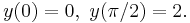
Without the boundary conditions, the general solution to this equation is

$y(x) = A \sin(x) + B \cos(x).\,$

From the boundary condition $y(0)=0$ one obtains

$0 = A \cdot 0 + B \cdot 1$

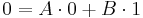
which implies that $B=0.$ From the boundary condition $y(\pi/2)=2$ one finds

$2 = A \cdot 1$

and so $A=2.$ One sees that imposing boundary conditions allowed one to determine a unique solution, which in this case is

$y(x)=2\sin(x). \,$

References

A. D. Polyanin and V. F. Zaitsev, Handbook of Exact Solutions for Ordinary Differential Equations (2nd edition), Chapman & Hall/CRC Press, Boca Raton, 2003. ISBN 1-58488-297-2.
A. D. Polyanin, Handbook of Linear Partial Differential Equations for Engineers and Scientists, Chapman & Hall/CRC Press, Boca Raton, 2002. ISBN 1-58488-299-9.

External links

Linear Partial Differential Equations: Exact Solutions and Boundary Value Problems at EqWorld: The World of Mathematical Equations.
Boundary value problem at Scholarpedia.