Atomic orbital

An atomic orbital is a mathematical function that describes the wave-like behavior of an electron in an atom. This function can be used to calculate the probability of finding any electron of an atom in any specific region around the atom's nucleus. The term "orbital" has become known as either the "mathematical function" or the "region" generated with the function.^[1] Specifically, atomic orbitals are the possible quantum states of an individual electron in the electron cloud around a single atom, as described by the function.

Electron atomic and molecular orbitals. The chart of orbitals (left) is arranged by increasing energy (see Madelung rule). Note that atomic orbits are functions of three variables (two angles, and the distance from the nucleus, r). These images are faithful to the angular component of the orbital, but not entirely representative of the orbital as a whole.

The idea that electrons moved in an orbit-like way inside an atom, was first suggested in 1904. From about 1913 to 1926 the electrons were thought to orbit the atomic nucleus much like the planets around the Sun. Explaining the behavior of the electron "orbits" was one of the driving forces behind the development of quantum mechanics. In quantum mechanics, atomic orbitals are described as wave functions over space, indexed by the n, l, and m quantum numbers of the orbital or by the names as used in electron configurations, as shown on the right. As electrons cannot be described as solid particles (like a planet), a more accurate analogy to the electron would be that of a large and often oddly-shaped atmosphere, the electron, distributed around a relatively tiny planet, which is the atomic nucleus. Because of the difference from classical mechanical orbits, the term "orbit" for electrons in atoms, has been replaced with the term orbital.

The orbital names (s, p, d, f, g, h,...) are derived from the characteristics of their spectroscopic lines: sharp, principal, diffuse, and fundamental, the rest being named in alphabetical order.

1 Orbital names
2 Formal quantum mechanical definition
3 Connection to uncertainty relation
4 Hydrogen-like atoms
5 Qualitative characterization
- 5.1 Limitations on the quantum numbers
6 The shapes of orbitals
- 6.1 Orbitals table
7 Orbital energy
8 Electron placement and the periodic table
- 8.1 Relativistic effects
9 See also
10 Notes
11 References
12 External links

Orbital names

Orbitals are given names in the form:

$X \, \mathrm{type}^y \$

where X is the energy level corresponding to the principal quantum number n, type is a lower-case letter denoting the shape or subshell of the orbital and it corresponds to the angular quantum number l, and y is the number of electrons in that orbital.

For example, the orbital 1s² (pronounced "one ess two") has two electrons and is the lowest energy level (n = 1) and has an angular quantum number of l = 0. In X-ray notation, the principal quantum number is given a letter associated with it. For n = 1, 2, 3, 4, 5 ....., the letters associated with those numbers are K, L, M, N, O .... respectively.

Formal quantum mechanical definition

In quantum mechanics, the state of an atom, i.e. the eigenstates of the atomic Hamiltonian, is expanded (see configuration interaction expansion and basis (linear algebra)) into linear combinations of anti-symmetrized products (Slater determinants) of one-electron functions. The spatial components of these one-electron functions are called atomic orbitals. (When one considers also their spin component, one speaks of atomic spin orbitals.)

In atomic physics, the atomic spectral lines correspond to transitions (quantum leaps) between quantum states of an atom. These states are labelled by a set of quantum numbers summarized in the term symbol and usually associated to particular electron configurations, i.e. by occupations schemes of atomic orbitals (e.g. 1s² 2s² 2p⁶ for the ground state of neon -- term symbol: ¹S₀).

This notation means that the corresponding Slater determinants have a clear higher weight in the configuration interaction expansion. The atomic orbital concept is therefore a key concept for visualizing the excitation process associated to a given transition. For example, one can say for a given transition that it corresponds to the excitation of an electron from an occupied orbital to a given unoccupied orbital. Nevertheless one has to keep in mind that electrons are fermions ruled by Pauli exclusion principle and cannot be distinguished from the other electrons in the atom. Moreover, it sometimes happens that the configuration interaction expansion converges very slowly and that one cannot speak about simple one-determinantal wave function at all. This is the case when electron correlation is large.

Fundamentally, an atomic orbital is a one-electron wavefunction, even though most electrons do not exist in one-electron atoms, and so the one-electron view is an approximation. When thinking about orbitals, we are often given an orbital vision which (even if it is not spelled out) is heavily influenced by this Hartree-Fock approximation, which is one way to reduce the complexities of molecular orbital theory.

Connection to uncertainty relation

Immediately after Heisenberg discovered his uncertainty relation, it was noted by Bohr that the existence of any sort of wave packet implies uncertainty in the wave frequency and wavelength, since a spread of frequencies is needed to create the packet itself. In quantum mechanics, where all particle momenta are associated with waves, it is the formation of such a wave packet which localizes the wave, and thus the particle, in space. In states where a quantum mechanical particle is bound, it must be localized as a wave packet, and the existence of the packet and its minimum size implies a spread and minimal value in particle wavelength, and thus also momentum and energy. In quantum mechanics, as a particle is localized to a smaller region in space, the associated compressed wave packet requires a larger and larger range of momenta, and thus larger kinetic energy. Thus, the binding energy to contain or trap a particle in a smaller region of space, increases without bound, as the region of space grows smaller. Particles cannot be restricted to a geometric point in space, since this would require an infinite particle momentum.

In chemistry, Schrödinger, Pauling, Mulliken and others noted that the consequence of Heisenberg's relation was that the electron, as a wave packet, could not be considered to have an exact location in its orbital. Max Born suggested that the electron's position needed to be described by a probability distribution which was connected with finding the electron at some point in the wave-function which described its associated wave packet. The new quantum mechanics did not give exact results, but only the probabilities for the occurrence of a variety of possible such results. Heisenberg held that the path of a moving particle has no meaning if we cannot observe it, as we cannot with electrons in an atom.

In the quantum picture of Heisenberg, Schrödinger and others, the Bohr atom number n for each orbital became known as an n-sphere in a three dimensional atom and was pictured as the mean energy of the probability cloud of the electron's wave packet which surrounded the atom.

Although Heisenberg used infinite sets of positions for the electron in his matrices, this does not mean that the electron could be anywhere in the universe. Rather there are several laws that show the electron must be in one localized probability distribution. An electron is described by its energy in Bohr's atom which was carried over to matrix mechanics. Therefore, an electron in a certain n-sphere had to be within a certain range from the nucleus depending upon its energy. This restricts its location.

Hydrogen-like atoms

Main article: Hydrogen-like atom

The simplest atomic orbitals are those that occur in an atom with a single electron, such as the hydrogen atom. In this case the atomic orbitals are the eigenstates of the hydrogen Hamiltonian. They can be obtained analytically (see hydrogen atom). An atom of any other element ionized down to a single electron is very similar to hydrogen, and the orbitals take the same form.

For atoms with two or more electrons, the governing equations can only be solved with the use of methods of iterative approximation. Orbitals of multi-electron atoms are qualitatively similar to those of hydrogen, and in the simplest models, they are taken to have the same form. For more rigorous and precise analysis, the numerical approximations must be used.

A given (hydrogen-like) atomic orbital is identified by unique values of three quantum numbers: n, l, and m_l. The rules restricting the values of the quantum numbers, and their energies (see below), explain the electron configuration of the atoms and the periodic table.

The stationary states (quantum states) of the hydrogen-like atoms are its atomic orbital. However, in general, an electron's behavior is not fully described by a single orbital. Electron states are best represented by time-depending "mixtures" (linear combinations) of multiple orbitals. See Linear combination of atomic orbitals molecular orbital method.

The quantum number n first appeared in the Bohr model. It determines, among other things, the distance of the electron from the nucleus; all electrons with the same value of n lie at the same distance. Modern quantum mechanics confirms that these orbitals are closely related. For this reason, orbitals with the same value of n are said to comprise a "shell". Orbitals with the same value of n and also the same value of l are even more closely related, and are said to comprise a "subshell".

Qualitative characterization

Limitations on the quantum numbers

An atomic orbital is uniquely identified by the values of the three quantum numbers, and each set of the three quantum numbers corresponds to exactly one orbital, but the quantum numbers only occur in certain combinations of values. The rules governing the possible values of the quantum numbers are as follows:

The principal quantum number n is always a positive integer. In fact, it can be any positive integer, but for reasons discussed below, large numbers are seldom encountered. Each atom has, in general, many orbitals associated with each value of n; these orbitals together are sometimes called electron shells.

The azimuthal quantum number $\ell$ is a non-negative integer. Within a shell where n is some integer n₀, $\ell$ ranges across all (integer) values satisfying the relation 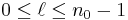$0 \le \ell \le n_0-1$ . For instance, the n = 1 shell has only orbitals with $\ell=0$ , and the n = 2 shell has only orbitals with $\ell=0$ , and $\ell=1$ . The set of orbitals associated with a particular value of $\ell$ are sometimes collectively called a subshell.

The magnetic quantum number $m_\ell$ is also always an integer. Within a subshell where $\ell$ is some integer $\ell_0$ , $m_\ell$ ranges thus: $-\ell_0 \le m_\ell \le \ell_0$ .

The above results may be summarized in the following table. Each cell represents a subshell, and lists the values of $m_\ell$ available in that subshell. Empty cells represent subshells that do not exist.

	$l=0$	1	2	3	4	...
$n=1$	$m_l=0$
2	0	-1, 0, 1
3	0	-1, 0, 1	-2, -1, 0, 1, 2
4	0	-1, 0, 1	-2, -1, 0, 1, 2	-3, -2, -1, 0, 1, 2, 3
5	0	-1, 0, 1	-2, -1, 0, 1, 2	-3, -2, -1, 0, 1, 2, 3	-4, -3, -2 -1, 0, 1, 2, 3, 4
...	...	...	...	...	...	...

Subshells are usually identified by their $n$ - and $\ell$ -values. $n$ is represented by its numerical value, but $\ell$ is represented by a letter as follows: 0 is represented by 's', 1 by 'p', 2 by 'd', 3 by 'f', and 4 by 'g'. For instance, one may speak of the subshell with $n=2$ and $\ell=0$ as a '2s subshell'.

The shapes of orbitals

The shapes of the first five atomic orbitals: 1s, 2s, 2p_x,2p_y, and 2p_z. The colors show the wavefunction phase.

Any discussion of the shapes of electron orbitals is necessarily imprecise, because a given electron, regardless of which orbital it occupies, can at any moment be found at any distance from the nucleus and in any direction due to the uncertainty principle.

However, the electron is much more likely to be found in certain regions of the atom than in others. Given this, a boundary surface can be drawn so that the electron has a high probability to be found anywhere within the surface, and all regions outside the surface have low values. The precise placement of the surface is arbitrary, but any reasonably compact determination must follow a pattern specified by the behavior of $\psi^2$ , the square of the wavefunction. This boundary surface is what is meant when the "shape" of an orbital is mentioned.

Generally speaking, the number $n$ determines the size and energy of the orbital: as $n$ increases, the size of the orbital increases.

Also in general terms, $\ell$ determines an orbital's shape, and $m_\ell$ its orientation. However, since some orbitals are described by equations in complex numbers, the shape sometimes depends on $m_\ell$ also.

The single $s$ -orbitals ( $\ell=0$ ) are shaped like spheres. For n=1 the sphere is "solid" (it is most dense at the center and fades exponentially outwardly), but for n=2 or more, each single s-orbital is composed of spherically symmetric surfaces which are nested shells (i.e., the "wave-structure" is radial, following a sinusoidal radial component as well). The $s$ -orbitals for all n numbers are the only orbitals with an anti-node (a region of high wave function density) at the center of the nucleus. All other orbitals (p, d, f, etc.) have angular momentum, and thus avoid the nucleus (having a wave node at the nucleus).

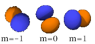
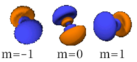
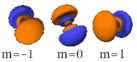
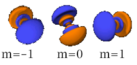
The three $p$ -orbitals have the form of two ellipsoids with a point of tangency at the nucleus (sometimes referred to as a dumbbell). The three $p$ -orbitals in each shell are oriented at right angles to each other, as determined by their respective values of $m_\ell$ .

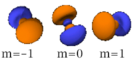
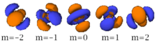
Four of the five $d$ -orbitals look similar, each with four pear-shaped balls, each ball tangent to two others, and the centers of all four lying in one plane, between a pair of axes. Three of these planes are the $xy$ -, $xz$ -, and $yz$ -planes, and the fourth has the centres on the $x$ and $y$ axes. The fifth and final $d$ -orbital consists of three regions of high probability density: a torus with two pear-shaped regions placed symmetrically on its $z$ axis.

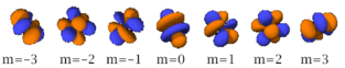
There are seven $f$ -orbitals, each with shapes more complex than those of the $d$ -orbitals.

For each s, p, d, f and g set of orbitals, the set of orbitals which composes it forms a spherically symmetrical set of shapes. For non-s orbitals, which have lobes, the lobes point in directions so as to fill space as symmetrically as possible for number of lobes which exist. For example, the three p orbitals have six lobes which are oriented to each of the six primary directions of 3-D space; for the 5 d orbitals, there are a total of 18 lobes, in which again six point in primary directions, and the 12 additional lobes fill the 12 gaps which exist between each pairs of these 6 primary axes.

The shapes of atomic orbitals in one-electron atom are related to 3-dimensional spherical harmonics.

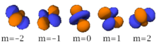
Orbitals table

This table shows all orbital configurations up to 7s, therefore it covers the simple electronic configuration for all elements from the periodic table up to radium.

	p (l=1)	d (l=2)	f (l=3)
n=1
n=2
n=3
n=4
n=5			. . .
n=6		. . .	. . .
n=7	. . .	. . .	. . .

Orbital energy

In atoms with a single electron (hydrogen-like atoms), the energy of an orbital (and, consequently, of any electrons in the orbital) is determined exclusively by $n$ . The $n=1$ orbital has the lowest possible energy in the atom. Each successively higher value of $n$ has a higher level of energy, but the difference decreases as $n$ increases. For high $n$ , the level of energy becomes so high that the electron can easily escape from the atom.

In atoms with multiple electrons, the energy of an electron depends not only on the intrinsic properties of its orbital, but also on its interactions with the other electrons. These interactions depend on the detail of its spatial probability distribution, and so the energy levels of orbitals depend not only on $n$ but also on $\ell$ . Higher values of $\ell$ are associated with higher values of energy; for instance, the 2p state is higher than the 2s state. When $\ell$ = 2, the increase in energy of the orbital becomes so large as to push the energy of orbital above the energy of the s-orbital in the next higher shell; when $\ell$ = 3 the energy is pushed into the shell two steps higher.

The energy sequence of the first 24 subshells is given in the following table. Each cell represents a subshell with $n$ and $\ell$ given by its row and column indices, respectively. The number in the cell is the subshell's position in the sequence. Empty cells represent sublevels that do not exist.

	$s$	$p$	$d$	$f$	$g$
1	1
2	2	3
3	4	5	7
4	6	8	10	13
5	9	11	14	17	21
6	12	15	18	22	26
7	16	19	23	27	31
8	20	24	28	32	36

Electron placement and the periodic table

Several rules govern the placement of electrons in orbitals (electron configuration). The first dictates that no two electrons in an atom may have the same set of values of quantum numbers (this is the Pauli exclusion principle). These quantum numbers include the three that define orbitals, as well as s, or spin quantum number. Thus, two electrons may occupy a single orbital, so long as they have different values of $s$ . However, only two electrons, because of their spin, can be associated with each orbital.

Additionally, an electron always tends to fall to the lowest possible energy state. It is possible for it to occupy any orbital so long as it does not violate the Pauli exclusion principle, but if lower-energy orbitals are available, this condition is unstable. The electron will eventually lose energy (by releasing a photon) and drop into the lower orbital. Thus, electrons fill orbitals in the order specified by the energy sequence given above.

This behavior is responsible for the structure of the periodic table. The table may be divided into several rows (called 'periods'), numbered starting with 1 at the top. The presently known elements occupy seven periods. If a certain period has number $i$ , it consists of elements whose outermost electrons fall in the $i$ th shell.

The periodic table may also be divided into several numbered rectangular 'blocks'. The elements belonging to a given block have this common feature: their highest-energy electrons all belong to the same $\ell$ -state (but the $n$ associated with that $\ell$ -state depends upon the period). For instance, the leftmost two columns constitute the 's-block'. The outermost electrons of Li and Be respectively belong to the 2s subshell, and those of Na and Mg to the 3s subshell.

The number of electrons in a neutral atom increases with the atomic number. The electrons in the outermost shell, or valence electrons, tend to be responsible for an element's chemical behavior. Elements that contain the same number of valence electrons can be grouped together and display similar chemical properties.

Relativistic effects

For elements with high atomic number Z, the effects of relativity become more pronounced, and especially so for s electrons, which move at relativistic velocities as they penetrate the screening electrons near the core of high Z atoms. This relativistic increase in momentum for high speed electrons causes a corresponding decrease in wavelength and contraction of 6s orbitals relative to 5d orbitals (by comparison to corresponding s and d electrons in lighter elements in the same column of the periodic table); this results in 6s valence electrons becoming lowered in energy.

Examples of significant physical outcomes of this effect include the lowered melting temperature of mercury (which results from 6s electrons not being available for metal bonding) and the golden color of gold and caesium (which result from narrowing of 6s to 5d transition energy to the point that visible light begins to be absorbed). See [1] and [2]).

In non-relativistic quantum mechanics, any atom with an atomic number greater than 137 would require 1s electrons to be traveling (have a mean velocity) faster than the speed of light. The significance of element 137, also known as untriseptium, was first pointed out by the physicist Richard Feynman. Element 137 is sometimes informally called feynmanium (symbol Fy). These properties of element 137 can be linked to the Fine Structure Constant, which is nearly $1/137$ .^[2]

However, this approximation is wrong in two ways. First, electrons do not actually move in orbits as predicted by the Bohr Model. Secondly, there is no problem with relativistic quantum mechanics, since arbitrarily large momentum does not imply arbitrarily large velocity, and electrons cannot exceed the speed of light no matter what their energy. The drastic effects caused by high electron energy happen only when the electron exceeds an energy of three or more times its rest energy. Under these circumstances, which require Z's in the 150's-- higher than can be found except in transient collision of heavy nuclei, the extra energy of the electron may be used to create electron-positron pairs.

Notes

↑ Daintith, J. (2004). Oxford Dictionary of Chemistry. New York: Oxford University Press. ISBN 0-19-860918-3.
↑ James G. Gilson (10 July 2008). "The fine structure constant, a 20th century mystery". Retrieved on 2008-07-15.

References

Tipler, Paul; Ralph Llewellyn (2003). Modern Physics (4 ed.). New York: W. H. Freeman and Company. ISBN 0-7167-4345-0.

External links

Guide to atomic orbitals
Covalent Bonds and Molecular Structure
Animation of the time evolution of an hydrogenic orbital
The Orbitron, a visualization of all common and uncommon atomic orbitals, from 1s to 7g
Grand table Still images of many orbitals
David Manthey's Orbital Viewer renders orbitals with n ≤ 30
Java orbital viewer applet
What does an atom look like? Orbitals in 3D

Atomic Models

Single atoms	Dalton model (Billiard Ball Model) · Thomson model (Plum Pudding Model) · Lewis model (Cubical Atom Model) · Nagaoka model (Saturnian Model) · Rutherford model (Planetary Model) · Bohr model (Rutherford–Bohr Model) · Bohr-Sommerfeld model (Refined Bohr Model) · Schrodinger model (Electron Cloud Model)

Atoms in solids	Drude model · Free electron model · Nearly-free electron model · Band structure · Density functional theory

Atoms in liquids	Liquid helium

Atoms in gases	Noble gas · Nascent hydrogen

Scientists	Felix Bloch · Niels Bohr · John Dalton · Paul Drude · Irving Langmuir · Gilbert N. Lewis · Hantaro Nagaoka · Ernest Rutherford · Erwin Schrödinger · Arnold Sommerfeld · J. J. Thomson