Arc length
Determining the length of an irregular arc segment — also called rectification of a curve — was historically difficult. Although many methods were used for specific curves, the advent of calculus led to a general formula that provides closed-form solutions in some cases.
Contents |
General approach

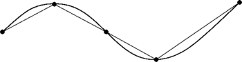
A curve in, say, the plane can be approximated by connecting a finite number of points on the curve using line segments to create a polygonal path. Since it is straightforward to calculate the length of each linear segment (using the theorem of Pythagoras in Euclidean space, for example), the total length of the approximation can be found by summing the lengths of each linear segment.
If the curve is not already a polygonal path, better approximations to the curve can be obtained by following the shape of the curve increasingly more closely. The approach is to use an increasingly larger number of segments of smaller lengths. The lengths of the successive approximations do not decrease and will eventually keep increasing – possibly indefinitely, but for smooth curves this will tend to a limit as the lengths of the segments get arbitrarily small.
For some curves there is a smallest number L that is an upper bound on the length of any polygonal approximation. If such a number exists, then the curve is said to be rectifiable and the curve is defined to have arc length L.
Definition
- See also: Curve#Lengths of curves
Let C be a curve in Euclidean (or, generally, a metric) space X = Rn, so C is the image of a continuous function f : [a, b] → X of the interval [a, b] into X.
From a partition a = t0 < t1 < … < tn−1 < tn = b of the interval [a, b] we obtain a finite collection of points f(t0), f(t1), …, f(tn−1), f(tn) on the curve C. Denote the distance from f(ti) to f(ti+1) by d(f(ti), f(ti+1)), which is the length of the line segment connecting the two points.
The arc length L of C is then defined to be
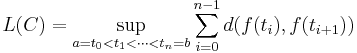
where the supremum is taken over all possible partitions of [a, b] and n is unbounded.
The arc length L is either finite or infinite. If L < ∞ then we say that C is rectifiable, and is non-rectifiable otherwise. This definition of arc length does not require that C is defined by a differentiable function.
Modern methods
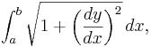
Consider a real function f(x) such that f(x) and f′(x) (its derivative with respect to x) are continuous on [a, b] . The length s of the part of the graph of f between x = a and x = b is found by the formula
![s = \int_{a}^{b} \sqrt { 1 + [f'(x)]^2 }\, dx.](/2009-wikipedia_en_wp1-0.7_2009-05/I/afe47a80440ceb225e21daf7caa71de5.png)
which is derived from the distance formula approximating the arc length with many small lines. As the number of line segments increases (to infinity by use of the integral) this approximation becomes an exact value.
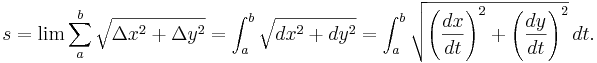
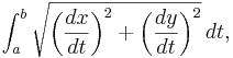
If a curve is defined parametrically by x = X(t) and y = Y(t), then its arc length between t = a and t = b is
![s = \int_{a}^{b} \sqrt { [X'(t)]^2 + [Y'(t)]^2 }\, dt.](/2009-wikipedia_en_wp1-0.7_2009-05/I/54ba060aefd5d2fbebbb3ab983e1ed65.png)
This is more clearly a consequence of the distance formula where instead of a Δx and Δy , we take the limit. A useful mnemonic is
If a function is defined in polar coordinates by r = f(θ) then the arc length is given by
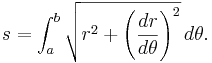
In most cases, including even simple curves, there are no closed-form solutions of arc length and numerical integration is necessary.
Curves with closed-form solution for arc length include the catenary, circle, cycloid, logarithmic spiral, parabola, semicubical parabola and (mathematically, a curve) straight line. The lack of closed form solution for the arc length of an elliptic arc led to the development of the elliptic integrals.
Derivation


In order to approximate the arc length of the curve, it is split into many linear segments. To make the value exact, and not an approximation, infinitely many linear elements are needed. This means that each element is infinitely small. This fact manifests itself later on when an integral is used.
Begin by looking at a representative linear segment (see image) and observe that its length (element of the arc length) will be the differential ds. We will call the horizontal element of this distance dx, and the vertical element dy.
The Pythagorean theorem tells us that
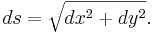
Since the function is defined in time, segments (ds) are added up across infintesimally small intervals of time (dt) yielding the integral
If y is a function of x, so that we could take t = x, then we have:
which is the arc length from x = a to x = b of the graph of the function ƒ.
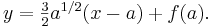
For example, the curve in this figure is defined by

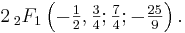
Subsequently, the arc length integral for values of t from −1 to 1 is
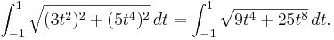
Using computational approximations, we can obtain a very accurate (but still approximate) arc length of 2.905. An expression in terms of the hypergeometric function can be obtained: it is
Another way to obtain the integral formula
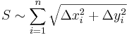
Suppose that we have a rectifiable curve given by a function f(x), and that we want to approximate the arc length S along f between two points a and b in that curve. We can construct a series of rectangle triangles whose concatenated hypotenuses "cover" the arch of curve chosen as it's shown in the figure. To make this a "more functional" method we can also demand that the bases of all those triangles were equal to Δ x, so that for each one an associated Δ y cathetus will exist, depending on the type of curve and on the chosen arch, being then every hypotenuse equal to 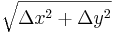 , as a result of the Pythagorean theorem. This way, an approximation of
  would be given by the summation of all those
  unfolded hypotenuses. Because of it we have that;
To continue, let's algebraically operate on the form in which we calculate every hypotenuse to come to a new expression:

Then, our previous result takes the following look:
Now, the smaller these segments are, the better our looked approximation is; they will be as small as we want doing that  tends to zero. This way, develops in
  , and every incremental quotient
  becomes into a general
  , that is by definition
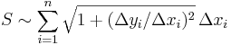
  . Given these changes, our previous approximation turns into a thinner and at this point exact summation; an integration of infinite infinitesimal segments;
![S = \lim_{\Delta x_i \to 0} \sum_{i=1}^\infty \sqrt { 1 + ({\Delta y_i / \Delta x_i})^2 }\,\Delta x_i = \int_{a}^{b} \sqrt { 1 + \left(\frac{dy}{dx}\right)^2 } \,dx = \int_{a}^{b} \sqrt{1 + \left [ f' \left ( x \right ) \right ] ^2} \, dx.](/2009-wikipedia_en_wp1-0.7_2009-05/I/67bcb7a0da370467e4742d26d75fc7ef.png)
Historical methods
Ancient
For much of the history of mathematics, even the greatest thinkers considered it impossible to compute the length of an irregular arc. Although Archimedes had pioneered a rectangular approximation for finding the area beneath a curve with his method of exhaustion, few believed it was even possible for curves to have definite lengths, as do straight lines. The first ground was broken in this field, as it often has been in calculus, by approximation. People began to inscribe polygons within the curves and compute the length of the sides for a somewhat accurate measurement of the length. By using more segments, and by decreasing the length of each segment, they were able to obtain a more and more accurate approximation.
1600s
In the 1600s, the method of exhaustion led to the rectification by geometrical methods of several transcendental curves: the logarithmic spiral by Evangelista Torricelli in 1645 (some sources say John Wallis in the 1650s), the cycloid by Christopher Wren in 1658, and the catenary by Gottfried Leibniz in 1691.
In 1659, Wallis credited William Neile's discovery of the first rectification of a nontrivial algebraic curve, the semicubical parabola.
Integral form
Before the full formal development of the calculus, the basis for the modern integral form for arc length was independently discovered by Hendrik van Heuraet and Pierre Fermat.
In 1659 van Heuraet published a construction showing that arc length could be interpreted as the area under a curve - this integral, in effect - and applied it to the parabola. In 1660, Fermat published a more general theory containing the same result in his De linearum curvarum cum lineis rectis comparatione dissertatio geometrica.

Building on his previous work with tangents, Fermat used the curve

whose tangent at x = a had a slope of

so the tangent line would have the equation
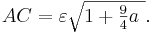
Next, he increased a by a small amount to a + ε, making segment AC a relatively good approximation for the length of the curve from A to D. To find the length of the segment AC, he used the Pythagorean theorem:
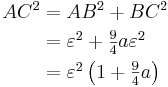
which, when solved, yields
In order to approximate the length, Fermat would sum up a sequence of short segments.
Curves with infinite length


As mentioned above, some curves are non-rectifiable, that is, they have infinite length. There are continuous curves for which any arc on the curve (containing more than a single point) has infinite length. An example of such a curve is the Koch curve. Another example of a curve with infinite length is the graph of the function defined by f(x) = x sin(1/x) for 0 ≤ x ≤ 1 and f(0) = 0. Sometimes the Hausdorff dimension and Hausdorff measure are used to "measure" the size of infinite length curves.
Generalization to (pseudo-)Riemannian manifolds
Let M be a (pseudo-)Riemannian manifold, γ : [0, 1] → M a curve in M and g the (pseudo-) metric tensor.
The length of γ is defined to be
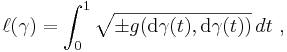
where dγ ∈ Tγ(t)M is the tangent vector of γ at t. The sign in the square root is chosen once for a given curve, to ensure that the square root is a real number. The positive sign is chosen for spacelike curves; in a pseudo-Riemannian manifold, the negative sign may be chosen for timelike curves.
In theory of relativity, arc-length of timelike curves (world lines) is the proper time elapsed along the world line.
See also
- Arc (geometry)
- Integral approximations
- Geodesics
References
- Farouki, Rida T. (1999). Curves from motion, motion from curves. In P-J. Laurent, P. Sablonniere, and L. L. Schumaker (Eds.), Curve and Surface Design: Saint-Malo 1999, pp.63-90, Vanderbilt Univ. Press. ISBN 0-8265-1356-5.
External links
- Math Before Calculus
- The History of Curvature
- Arc Length by Ed Pegg, Jr., The Wolfram Demonstrations Project, 2007.
- Calculus Study Guide – Arc Length (Rectification)
- Famous Curves Index The MacTutor History of Mathematics archive
- Arc Length Approximation by Chad Pierson, Josh Fritz, and Angela Sharp, The Wolfram Demonstrations Project.
- Length of a Curve Experiment Illustrates numerical solution of finding length of a curve.