Ampère's circuital law

Electromagnetism

Electrostatics
· Electric charge · Coulomb’s law · Electric field · Electric flux · Gauss’ law · Electric potential · Electrostatic induction · Electric dipole moment ·

Magnetostatics
· Ampère’s law · Electric current · Magnetic field · Magnetic flux · Biot–Savart law · Magnetic dipole moment · Gauss’s law for magnetism ·

Electrodynamics
· Free space · Lorentz force law · EMF · Electromagnetic induction · Faraday’s law · Displacement current · Maxwell’s equations · EM field · Electromagnetic radiation · Liénard-Wiechert Potentials · Maxwell tensor · Eddy current ·

Electrical Network
· Electrical conduction · Electrical resistance · Capacitance · Inductance · Impedance · Resonant cavities · Waveguides ·

Covariant formulation
· Electromagnetic tensor · EM Stress-energy tensor · Four-current · Four-potential ·

Scientists
· Ampère · Coulomb · Faraday · Heaviside · Henry · Hertz · Lorentz · Maxwell · Tesla · Weber ·

In classical electromagnetism, Ampère's circuital law, discovered by André-Marie Ampère in 1826 [1], relates the integrated magnetic field around a closed loop to the electric current passing through the loop. It is one of Maxwell's equations, which form the basis of classical electromagnetism.

1 Original Ampère's circuital law
- 1.1 Integral form
- 1.2 Differential form
2 Note on free current versus bound current
3 Shortcomings of the original formulation of Ampère's circuital law
- 3.1 Displacement current
4 Extending the original law: the Maxwell-Ampère equation
- 4.1 Proof of equivalence
5 Ampère's law in cgs units
6 In-line references and notes
7 Further reading
8 External links
9 See also

Original Ampère's circuital law

An electric current produces a magnetic field.

In its historically original form, Ampère's Circuital Law relates the magnetic field to its electric current source. The law can be written in two forms, the "integral form" and the "differential form". The forms are equivalent, and related by the Kelvin-Stokes theorem.

Integral form

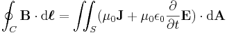
In SI units, (the version in cgs units is in a later section), the "integral form" of the original Ampère's circuital law is:^[1]^[2]

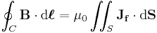
$\oint_C \mathbf{B} \cdot \mathrm{d}\boldsymbol{\ell} = \mu_0 \iint_S \mathbf{J_f} \cdot \mathrm{d}\mathbf{S}$

or equivalently,

$\oint_C \mathbf{B} \cdot \mathrm{d}\boldsymbol{\ell} = \mu_0 I_{\mathrm{enc}}$

where:

$\oint_C$ is the closed line integral around the closed curve C.
$\mathbf{B}$ is the magnetic field in tesla.
$\cdot$ is the vector dot product.
$\mathrm{d}\boldsymbol{\ell}$ is an infinitesimal element (differential) of the curve C (i.e. a vector with magnitude equal to the length of the infinitesimal line element, and direction given by the tangent to the curve C, see below),
$\iint_S$ denotes an integral over the surface S enclosed by the curve C (see below). The double integral sign is meant simply to denote that the integral is two-dimensional in nature.
$\mu_0 \!\$ is the magnetic constant also called the absolute permeability of free space.
$\mathbf{J_f}$ is the free current density through the surface S enclosed by the curve C
$\mathrm{d}\mathbf{S} \!\$ is the vector area of an infinitesimal element of surface S (that is, a vector with magnitude equal to the area of the infinitesimal surface element, and direction normal to surface S. The direction of the normal must correspond with the orientation of C by the right hand rule, see below for further discussion),
$I_{\mathrm{enc}} \!\$ is the net free current that penetrates through the surface S.

There are a number of ambiguities in the above definitions that warrant elaboration.

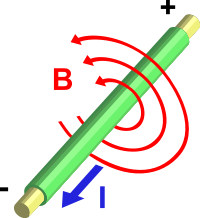
First, three of these terms are associated with sign ambiguities: the line integral $\oint_C$ could go around the loop in either direction (clockwise or counterclockwise); the vector area $\mathrm{d}\mathbf{S}$ could point in either of the two directions normal to the surface; and $I_{\mathrm{enc}}$ is the net current passing through the surface S, meaning the current passing through in one direction, minus the current in the other direction--but either direction could be chosen as positive. These ambiguities are resolved by the right-hand rule: When the index-finger of the right-hand points along the direction of line-integration, the outstretched thumb points in the direction that must be chosen for the vector area $\mathrm{d}\mathbf{S}$ , and current passing in that same direction must be counted as positive. The right hand grip rule can also be used to determine the signs.

Second, there are infinitely many possible surfaces S that have the curve C as their border. (Imagine a soap film on a wire loop, which can be deformed by blowing gently at it.) Which of those surfaces is to be chosen? If the loop does not lie in a single plane, for example, there is no one obvious choice. The answer is that it does not matter; it can be proven that any surface with boundary C can be chosen.

Differential form

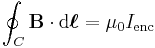
By the Kelvin-Stokes theorem, this equation can also be written in a "differential form". Again, this equation only applies in the case where the electric field is constant in time; see below for the more general form. In SI units, the equation states:

$\mathbf{\nabla} \times \mathbf{B} = \mu_0 \mathbf{J_f}$

where

$\mathbf{\nabla} \times \!\$ is the curl operator.

Note on free current versus bound current

The electric current that arises in the simplest textbook situations would be classified as "free current"—for example, the current that passes through a wire or battery. In contrast, "bound current" arises in the context of bulk materials that can be magnetized and/or polarized. (All materials can to some extent.)

When a material is magnetized (for example, by placing it in an external magnetic field), the electrons remain bound to their respective atoms, but behave as if they were orbiting the nucleus in a particular direction, creating a microscopic current. When the currents from all these atoms are put together, they create the same effect as a macroscopic current, circulating perpetually around the magnetized object. This magnetization current J_M is one contribution to "bound current".

The other source of bound current is bound charge. When an electric field is applied, the positive and negative bound charges can separate over atomic distances in polarizable materials, and when the bound charges move, the polarization changes, creating another contribution to the "bound current", the polarization current J_P.

The total current density J due to free and bound charges is then:

$\mathbf{J} =\mathbf{J_f +J_M +J_P} \ ,$

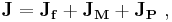
with J_f the "free" or "conduction" current density.

All current is fundamentally the same, microscopically. Nevertheless, there are often practical reasons for wanting to treat bound current differently from free current. For example, the bound current usually originates over atomic dimensions, and one may wish to take advantage of a simpler theory intended for larger dimensions. The result is that the more microscopic Ampère's law, expressed in terms of B and the microscopic current (which includes free, magnetization and polarization currents), is sometimes put into the equivalent form below in terms of H and the free current only. For a detailed definition of free current and bound current, and the proof that the two formulations are equivalent, see the "proof" section below.

Shortcomings of the original formulation of Ampère's circuital law

There are two important issues regarding Ampère's law which require closer scrutiny. First, there is an issue regarding the continuity equation for electrical charge. There is a theorem in vector calculus which states that the divergence of a curl must always be zero. Hence ∇·(∇×B) = 0 and so the original Ampère's law implies that ∇·J = 0. But in general ∇·J = −∂ρ / ∂t, which is non-zero for a time-varying charge density. An example occurs in a capacitor circuit where time-varying charge densities exist on the plates. ^[3]^[4]^[5]^[6]^[7]

Second, there is an issue regarding the propagation of electromagnetic waves. For example, in free space, where J = 0, Ampère's law implies that∇×B = 0, but instead ∇×B = −(1/c²) ∂E / ∂t.

To treat these situations, the contribution of displacement current must be added to the "free current" term in Ampère's law.

James Clerk Maxwell conceived of displacement current as a polarization current in the dielectric vortex sea which he used to model the magnetic field hydrodynamically and mechanically.^[8] He added this displacement current to Ampère's circuital law at equation (112) in his 1861 paper On Physical Lines of Force.

Displacement current

Main article: Displacement current

In free space, the displacement current is related to the time rate of change of electric field.

In a dielectric the above contribution to displacement current is present too, but a major contribution to the displacement current is related to the polarization of the individual molecules of the dielectric material. Even though charges cannot flow freely in a dielectric, the charges in molecules can move a little under the influence of an electric field. The positive and negative charges in molecules separate under the applied field, causing an increase in the state of polarization, expressed as the polarization density P. A changing state of polarization is equivalent to a current.

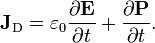
Both contributions to the displacement current are combined by defining the displacement current as:^[3]

$\mathbf{J_D} = \frac {\partial}{\partial t} \mathbf D (\boldsymbol r , \ t) \ ,$

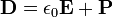
where the electric displacement field is defined as:

$\mathbf{D} = \varepsilon_0 \mathbf{E} + \mathbf{P}\ ,$

where ε₀ is the electric constant and P is the polarization density. Substituting this form for D in the expression for displacement current, it has two components:

$\mathbf{J}_\mathrm{D} = \varepsilon_0 \frac{\partial \mathbf{E}}{\partial t} + \frac{\partial \mathbf{P}}{\partial t}.$

The first term on the right hand side is present everywhere, even in a vacuum. It doesn't involve any actual movement of charge, but it nevertheless has an associated magnetic field, as if it were an actual current. Some authors apply the name displacement current to only this contribution.^[9]

The second term on the right hand side is the displacement current as originally conceived by Maxwell, associated with the polarization of the individual molecules of the dielectric material.

Maxwell's original explanation for displacement current focused upon the situation that occurs in dielectric media. In the modern post-aether era, the concept has been extended to apply to situations with no material media present, for example, to the vacuum between the plates of a charging vacuum capacitor. The displacement current is justified today because it serves several requirements of an electromagnetic theory: correct prediction of magnetic fields in regions where no free current flows; prediction of wave propagation of electromagnetic fields; and conservation of electric charge in cases where charge density is time-varying. For greater discussion see Displacement current.

Extending the original law: the Maxwell-Ampère equation

Next Ampère's equation is extended by including the polarization current, thereby remedying the limited applicability of the original Ampère's circuital law.

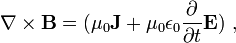
Treating free charges separately from bound charges, Ampère's equation including Maxwell's correction in terms of the H-field is (the H-field is used because it includes the magnetization currents, so J_M does not appear explicitly, see H-field and also Note):^[10]

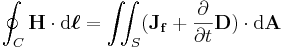
$\oint_C \mathbf{H} \cdot \mathrm{d}\boldsymbol{\ell} = \iint_S (\mathbf{J_f}+ \frac{\partial }{\partial t}\mathbf{D}) \cdot \mathrm{d} \mathbf{A}$

(integral form), where:

H is the magnetic H field (also called "auxiliary magnetic field", "magnetic field intensity", or just "magnetic field",
D is the electric displacement field
J_f is the enclosed conduction current or free current density,

or (differential form):

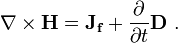
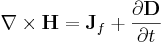
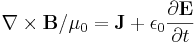
$\mathbf{\nabla}\times \mathbf{H} = \mathbf{J_f}+\frac{\partial }{\partial t}\mathbf{D} \ .$

On the other hand, treating all charges on the same footing (disregarding whether they are bound or free charges), the generalized Ampère's equation (or Maxwell-Ampère equation) is (see the "proof" section below):

$\oint_C \mathbf{B} \cdot \mathrm{d}\boldsymbol{\ell} = \iint_S (\mu_0 \mathbf{J}+ \mu_0 \epsilon_0 \frac{\partial }{\partial t}\mathbf{E}) \cdot \mathrm{d} \mathbf{A}$

(integral form), or (differential form):

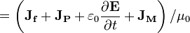
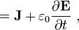
$\mathbf{\nabla}\times \mathbf{B} = (\mu_0\mathbf{J}+\mu_0 \epsilon_0 \frac{\partial }{\partial t}\mathbf{E}) \ ,$

where J includes magnetization current density^[11] as well as conduction and polarization current densities. That is, the current density on the right side of the Ampère-Maxwell equation is:

$\mathbf{J_f+J_D +J_M} = \mathbf{J_f +J_P +J_M} + \varepsilon_0 \frac {\partial \mathbf{E}}{\partial t} = \mathbf{J}+ \varepsilon_0 \frac {\partial \mathbf{E}}{\partial t} \ ,$

where current density J_D is the displacement current, and J is the current density contribution actually due to movement of charges, both free and bound. Because ∇·D = ρ, the charge continuity issue with Ampère's original formulation is no longer a problem.^[12] Because of the term in ε₀∂E / ∂t, wave propagation in free space now is possible.

With the addition of the displacement current, Maxwell was able to hypothesize (correctly) that light was a form of electromagnetic wave. See electromagnetic wave equation for a discussion of this important discovery.

Proof of equivalence

Proof that the formulations of Ampère's law in terms of free current are equivalent to the formulations involving total current.

In this proof, we will show that the equation

$\nabla\times \mathbf{H} = \mathbf{J}_f + \frac{\partial \mathbf{D}}{\partial t}$

is equivalent to the equation

$\mathbf{\nabla} \times \mathbf{B}/\mu_0 = \mathbf{J} + \epsilon_0 \frac{\partial \mathbf{E}}{\partial t}$

Note that we're only dealing with the differential forms, not the integral forms, but that is sufficient since the differential and integral forms are equivalent in each case, by the Kelvin-Stokes theorem.

We introduce the polarization density P, which has the following relation to E and D:

$\mathbf{D}=\epsilon_0 \mathbf{E} + \mathbf{P}$

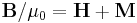
Next, we introduce the magnetization density M, which has the following relation to B and H:

$\mathbf{B}/\mu_0 = \mathbf{H} + \mathbf{M}$

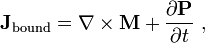
and the following relation to the bound current:

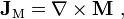
$\mathbf{J}_{\mathrm{bound}} = \nabla\times\mathbf{M} + \frac{\partial \mathbf{P}}{\partial t}\ ,$

$=\mathbf{J}_{\mathrm{M}}+\mathbf{J}_{\mathrm{P}}\ ,$

where

$\mathbf{J}_{\mathrm{M}} = \nabla\times\mathbf{M} \ ,$

is called the magnetization current density, and

$\mathbf{J}_{\mathrm{P}} = \frac{\partial \mathbf{P}}{\partial t}\ ,$

is the polarization current density. Taking the equation for B:

$\mathbf{\nabla} \times \mathbf{B}/\mu_0 = \mathbf{\nabla} \times \left( \mathbf {H+M} \right)/\mu_0$

$=\left (\mathbf{\nabla} \times \mathbf H + \mathbf{J_M} \right)/\mu_0$

$=\left ( \mathbf{J_f} + \mathbf{J_P} +\varepsilon_0 \frac{\partial \mathbf E}{\partial t} + \mathbf{J_M}\right)/\mu_0$

Consequently, referring to the definition of the bound current:

$\mathbf{\nabla} \times \mathbf{B} =\mathbf{J_f}+ \mathbf{J}_{\mathrm{bound}} + \varepsilon_0 \frac{\partial \mathbf E }{\partial t}$

$=\mathbf{J} + \varepsilon_0 \frac{\partial \mathbf E}{\partial t} \ ,$

as was to be shown.

Ampère's law in cgs units

In cgs units, the integral form of the equation, including Maxwell's correction, reads

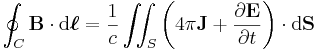
$\oint_C \mathbf{B} \cdot \mathrm{d}\boldsymbol{\ell} = \frac{1}{c} \iint_S \left(4\pi\mathbf{J}+\frac{\partial \mathbf{E}}{\partial t}\right) \cdot \mathrm{d}\mathbf{S}$

where c is the speed of light.

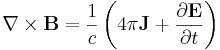
The differential form of the equation (again, including Maxwell's correction) is

$\mathbf{\nabla} \times \mathbf{B} = \frac{1}{c}\left(4\pi\mathbf{J}+\frac{\partial \mathbf{E}}{\partial t}\right)$

In-line references and notes

↑ Heinz E Knoepfel (2000). Magnetic Fields: A comprehensive theoretical treatise for practical use. Wiley. p. p. 4. ISBN 0471322059. http://books.google.com/books?id=1n7NPasgh0sC&pg=PA210&dq=isbn:0471322059#PPA4,M1.
↑ George E Owen (2003). Electromagnetic Theory (Reprint of 1963 edition ed.). Courier-Dover Publications. p. p. 213. ISBN 0486428303. http://books.google.com/books?id=VLm_dqhZUOYC&pg=PA213&dq=%22Ampere%27s+circuital+law%22&lr=&as_brr=0#PPA213,M1.
↑ ^3.0 ^3.1 John David Jackson (1999). Classical Electrodynamics (3rd Edition ed.). Wiley. p. p. 238. ISBN 047130932X.
↑ David J Griffiths (1999). Introduction to Electrodynamics (3rd Edition ed.). Pearson/Addison-Wesley. p. pp. 322-323. ISBN 013805326X. http://books.google.com/books?id=w0YgJgAACAAJ&dq=isbn:013805326X.
↑ George E Owen. op. cit.. p. p. 285. ISBN 0486428303. http://books.google.com/books?id=VLm_dqhZUOYC&pg=PA213&dq=%22Ampere%27s+circuital+law%22&lr=&as_brr=0#PPA285,M1.
↑ J Billingham, A C King (2006). Wave Motion. Cambridge University Press. p. p. 179. ISBN 0521634504. http://books.google.com/books?id=bNePaHM20LQC&pg=PA179&dq=displacement+%22ampere%27s+law%22&lr=&as_brr=0.
↑ JC Slater and NH Frank (1969). Electromagnetism (Reprint of 1947 edition ed.). Courier Dover Publications. p. p. 83. ISBN 0486622630. http://books.google.com/books?id=GYsphnFwUuUC&pg=PA83&dq=displacement+%22ampere%27s+law%22&lr=&as_brr=0#PPA83,M1.
↑ Daniel M. Siegel (2003). Innovation in Maxwell's Electromagnetic Theory: Molecular Vortices, Displacement Current, and Light. Cambridge University Press. p. pp. 96-98. ISBN 0521533295. http://books.google.com/books?id=AbQq85U8K0gC&pg=PA97&dq=Ampere%27s+circuital+law+%22displacement+current%22&lr=&as_brr=0#PPA97,M1.
↑ For example, see David J Griffiths. 'op. cit.'. p. p. 323. ISBN 013805326X. and Tai L Chow (2006). Introduction to Electromagnetic Theory. Jones & Bartlett. p. p. 204. ISBN 0763738271. http://books.google.com/books?id=dpnpMhw1zo8C&pg=PA153&dq=isbn:0763738271#PPA204,M1.
↑ Mircea S. Rogalski, Stuart B. Palmer (2006). Advanced University Physics. CRC Press. p. p. 267. ISBN 1584885114. http://books.google.com/books?id=rW95PWh3YbkC&pg=PA266&dq=displacement+%22Ampere%27s+circuital+law%22&lr=&as_brr=0#PPA267,M1.
↑ Stuart B Palmer & Mircea S. Rogalski (2006). Advanced University Physics. CRC Press. p. p. 251. ISBN 1584885114. http://books.google.com/books?id=rW95PWh3YbkC&printsec=frontcover#PPA251,M1.
↑ The magnetization current can be expressed as the curl of the magnetization, so its divergence is zero and it does not contribute to the continuity equation. See magnetization current.

External links

Simple Nature by Benjamin Crowell Ampere's law from an online textbook
MISN-0-138 Ampere's Law (PDF file) by Kirby Morgan for Project PHYSNET.
MISN-0-145 The Ampere-Maxwell Equation; Displacement Current (PDF file) by J.S. Kovacs for Project PHYSNET.
The Ampère's Law Song (PDF file) by Walter Fox Smith; Main page, with recordings of the song.
A Dynamical Theory of the Electromagnetic Field Maxwell's paper of 1864